Introduction
Machine Learning has become one of the most influential technologies of the modern digital era, powering applications that range from search engines and recommendation systems to medical diagnosis, financial forecasting, autonomous vehicles, and intelligent IoT systems. At the heart of many of these applications lies supervised learning, a fundamental branch of machine learning where models learn directly from labeled data to make accurate predictions on unseen examples.
Supervised learning algorithms operate on a simple but powerful idea: given historical data where both the inputs and the correct outputs are known, a model can learn the underlying relationship between them. Once trained, this model can generalize that knowledge to predict outcomes for new data. This paradigm makes supervised learning particularly valuable in real-world scenarios where past observations and outcomes are available, such as predicting house prices, classifying emails as spam or not, diagnosing diseases, detecting fraud, or forecasting customer behavior.
However, despite their widespread use, supervised learning algorithms are often treated as “black boxes” by beginners. Many learners know how to call a function from a library like scikit-learn, but struggle to understand why an algorithm works, how it makes decisions, and when it should be preferred over another. Choosing an inappropriate algorithm, misinterpreting its assumptions, or ignoring its limitations can lead to poor model performance, biased predictions, or misleading conclusions.
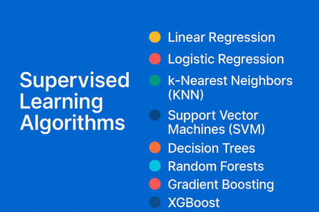
This tutorial is designed to bridge that gap between theory and practice. It provides a clear, structured, and in-depth exploration of the most important supervised learning algorithms, starting from simple linear models and gradually progressing toward powerful ensemble methods such as Random Forests, Gradient Boosting, and XGBoost. Each algorithm is explained from multiple complementary perspectives:
- Intuition, to build a conceptual understanding of how the model thinks and learns
- Mathematical foundations, presented at a light to medium level, to clarify the underlying principles without overwhelming the reader
- Python implementations, using industry-standard libraries, to show how these models are applied in practice
- Advantages and limitations, to help you make informed decisions when selecting a model
- Real-world use cases, connecting theory to concrete applications across different domains
Rather than focusing on isolated formulas or abstract definitions, this tutorial emphasizes practical understanding and model selection. You will learn not only how to train a model, but also how to reason about its behavior, interpret its outputs, and recognize situations where it may fail. This approach is essential for building reliable, scalable, and ethical machine learning systems.
The tutorial is suitable for:
- Beginners who know basic Python and want a solid foundation in supervised learning
- Engineering and data science students seeking a clear and structured reference
- Developers and practitioners who want to strengthen their understanding of model behavior before deploying ML solutions
By the end of this tutorial, you will have a strong conceptual and practical grasp of supervised learning algorithms, enabling you to confidently choose, implement, and evaluate models for real-world machine learning problems. This knowledge will also prepare you for more advanced topics such as deep learning, model optimization, and MLOps workflows.
1. What is Supervised Learning?
Supervised learning is a category of machine learning where the model learns a mapping between input features (X) and known target labels (y) using labeled data.
$(X, y) \rightarrow \text{Model} \rightarrow \hat{y}$
Main Tasks
- Regression → Predict continuous values
- Classification → Predict discrete classes
1️⃣ Linear Regression
Intuition
Linear Regression models the relationship between variables by fitting a straight line (or hyperplane) that minimizes the error between predictions and real values.
“Find the line that best explains the data.”
Mathematical Explanation
Model:
$\beta_0 + \beta_1 x_1 + \beta_2 x_2 + \dots + \beta_n x_n$
Loss function (Mean Squared Error):
$J(\beta) = \frac{1}{n}\sum_{i=1}^{n}(y_i - \hat{y}_i)^2$
Optimization is done using Normal Equation or Gradient Descent.
Python Implementation
from sklearn.linear_model import LinearRegression
from sklearn.model_selection import train_test_split

X = [[1], [2], [3], [4]]
y = [2, 4, 6, 8]

model = LinearRegression()
model.fit(X, y)

print(model.predict([[5]]))
Pros & Cons
Pros
- Simple and interpretable
- Fast to train
- Good baseline model
Cons
- Assumes linearity
- Sensitive to outliers
- Poor performance on complex data
Real-World Use Cases
- House price prediction
- Sales forecasting
- Economic trend analysis
2️⃣ Logistic Regression
Intuition
Despite its name, Logistic Regression is a classification algorithm.
It models the probability that an input belongs to a class.
Mathematical Explanation
Sigmoid function:
$\sigma(z) = \frac{1}{1 + e^{-z}}$
Decision rule:
$P(y=1|x) > 0.5 \Rightarrow \text{Class 1}$
Loss function: Log Loss (Cross-Entropy)
Python Implementation
from sklearn.linear_model import LogisticRegression

X = [[1], [2], [3], [4]]
y = [0, 0, 1, 1]

model = LogisticRegression()
model.fit(X, y)

print(model.predict([[2.5]]))
Pros & Cons
Pros
- Outputs probabilities
- Interpretable coefficients
- Works well for linearly separable data
Cons
- Limited to linear decision boundaries
- Struggles with complex patterns
Real-World Use Cases
- Spam detection
- Credit approval
- Medical diagnosis (yes/no)
3️⃣ k-Nearest Neighbors (KNN)
Intuition
KNN predicts based on the labels of the nearest neighbors in the feature space.
“Tell me who your neighbors are, and I’ll tell you who you are.”
Mathematical Explanation
Distance metric (usually Euclidean):
$d(x, x_i) = \sqrt{\sum (x - x_i)^2}$
Classification by majority vote among k neighbors.
Python Implementation
from sklearn.neighbors import KNeighborsClassifier

model = KNeighborsClassifier(n_neighbors=3)
model.fit(X, y)

print(model.predict([[3]]))
Pros & Cons
Pros
- No training phase
- Simple and intuitive
- Non-parametric
Cons
- Slow for large datasets
- Sensitive to feature scaling
- Memory intensive
Real-World Use Cases
- Recommendation systems
- Pattern recognition
- Image classification (small datasets)
4️⃣ Support Vector Machines (SVM)
Intuition
SVM finds the optimal hyperplane that maximizes the margin between classes.
Mathematical Explanation
Optimization objective:
$\min \frac{1}{2}||w||^2$
Subject to:
$y_i(w \cdot x_i + b) \geq 1$
Kernel trick enables non-linear boundaries.
Python Implementation
from sklearn.svm import SVC

model = SVC(kernel='rbf')
model.fit(X, y)

print(model.predict([[3]]))
Pros & Cons
Pros
- Effective in high dimensions
- Kernel flexibility
- Robust to overfitting
Cons
- Computationally expensive
- Harder to interpret
- Sensitive to parameter tuning
Real-World Use Cases
- Face recognition
- Bioinformatics
- Text classification
5️⃣ Decision Trees
Intuition
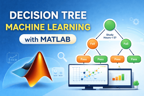
Decision Trees split data based on if-then rules until a decision is made.
Mathematical Explanation
Splitting criteria:
- Gini Index
- Entropy (Information Gain)
Entropy:
$H(S) = -\sum p_i \log_2 p_i$
Python Implementation
from sklearn.tree import DecisionTreeClassifier

model = DecisionTreeClassifier(max_depth=3)
model.fit(X, y)

print(model.predict([[3]]))
Pros & Cons
Pros
- Highly interpretable
- Handles non-linear data
- No feature scaling required
Cons
- Prone to overfitting
- Unstable with small data changes
Real-World Use Cases
- Rule-based systems
- Customer segmentation
- Credit risk analysis
6️⃣ Random Forests
Intuition
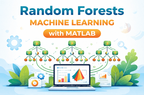
Random Forest combines multiple decision trees to reduce variance.
“Wisdom of the crowd.”
Mathematical Explanation
- Bagging (Bootstrap Aggregation)
- Random feature selection
Prediction = majority vote / average
Python Implementation
from sklearn.ensemble import RandomForestClassifier

model = RandomForestClassifier(n_estimators=100)
model.fit(X, y)

print(model.predict([[3]]))
Pros & Cons
Pros
- High accuracy
- Robust to overfitting
- Handles missing values
Cons
- Less interpretable
- Larger model size
Real-World Use Cases
- Fraud detection
- Feature importance analysis
- Industrial ML systems
7️⃣ Gradient Boosting
Intuition
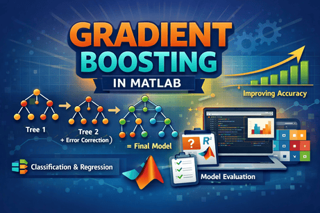
Models are trained sequentially, each correcting the errors of the previous one.
Mathematical Explanation
Additive model:
$F_m(x) = F_{m-1}(x) + \gamma h_m(x)$
Optimizes a differentiable loss function.
Python Implementation
from sklearn.ensemble import GradientBoostingClassifier

model = GradientBoostingClassifier()
model.fit(X, y)

print(model.predict([[3]]))
Pros & Cons
Pros
- High predictive power
- Handles complex patterns
Cons
- Slower training
- Sensitive to hyperparameters
Real-World Use Cases
- Web ranking
- Financial modeling
- Predictive analytics
8️⃣ XGBoost (Extreme Gradient Boosting)
Intuition
XGBoost is an optimized and regularized version of gradient boosting.
Mathematical Explanation
Objective function:
$\text{Loss} + \Omega(\text{Model})$
Regularization controls complexity.
Python Implementation
from xgboost import XGBClassifier

model = XGBClassifier(use_label_encoder=False, eval_metric='logloss')
model.fit(X, y)

print(model.predict([[3]]))
Pros & Cons
Pros
- State-of-the-art performance
- Built-in regularization
- Handles missing data
Cons
- Complex tuning
- Less interpretable
Real-World Use Cases
- Kaggle competitions
- Credit scoring
- Large-scale ML systems📊 Algorithm Comparison Summary
| Algorithm | Type | Complexity | Interpretability |
|---|---|---|---|
| Linear Regression | Regression | Low | High |
| Logistic Regression | Classification | Low | High |
| KNN | Both | Medium | Medium |
| SVM | Both | High | Medium |
| Decision Tree | Both | Medium | High |
| Random Forest | Both | High | Medium |
| Gradient Boosting | Both | High | Low |
| XGBoost | Both | Very High | Low |










💬 Comments
No comments yet. Be the first to comment!
Login to comment.