Model Evaluation & Metrics

By echrif | décembre 23, 2025

This tutorial explains how to evaluate machine learning models using the most important regression and classification metrics. It covers MSE, RMSE, MAE, and R² for regression, as well as Accuracy, Precision, Recall, F1-score, Confusion Matrix, and ROC-AUC for classification, with clear explanations and practical visualizations using Matplotlib and Seaborn.

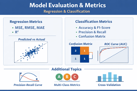
When you train a model, you need objective ways to judge how good (or bad) it is. Metrics help you compare models, tune hyperparameters, and understand tradeoffs (like missing positives vs. triggering false alarms).

We’ll cover:

Regression: MSE, RMSE, MAE, R²
Classification: Accuracy, Precision, Recall, F1, Confusion Matrix, ROC-AUC
Visualizations: Matplotlib + Seaborn (confusion matrix heatmap, ROC curve, residual plots)

1) Setup

pip install numpy pandas matplotlib seaborn scikit-learn

import numpy as np
import matplotlib.pyplot as plt
import seaborn as sns

from sklearn.model_selection import train_test_split
from sklearn.linear_model import LinearRegression, LogisticRegression
from sklearn.metrics import (
    mean_squared_error, mean_absolute_error, r2_score,
    accuracy_score, precision_score, recall_score, f1_score,
    confusion_matrix, roc_curve, roc_auc_score
)

sns.set_theme(style="whitegrid")
np.random.seed(42)

2) Regression Metrics

Regression predicts a continuous value (price, temperature, demand…).

2.1 MSE (Mean Squared Error)

$\text{MSE} = \frac{1}{n}\sum_{i=1}^{n}(y_i - \hat{y}_i)^2$

Penalizes large errors heavily (because of squaring).
Sensitive to outliers.

2.2 RMSE (Root Mean Squared Error)

$\text{RMSE} = \sqrt{\text{MSE}}$

Same unit as the target (e.g., dollars).
Still sensitive to outliers.

2.3 MAE (Mean Absolute Error)

$\text{MAE} = \frac{1}{n}\sum_{i=1}^{n}|y_i - \hat{y}_i|$

More robust to outliers than MSE/RMSE.
Interpretable: “average absolute mistake.”

2.4 R² (Coefficient of Determination)

$R^2 = 1 - \frac{\sum (y_i - \hat{y}_i)^2}{\sum (y_i - \bar{y})^2}$

Measures how much variance is explained vs. predicting the mean.
1.0 perfect, 0.0 same as mean predictor, < 0 worse than mean predictor.

2.5 Regression Example + Visualizations

We’ll build a synthetic regression dataset, train a model, compute metrics, and visualize residuals.

# Synthetic regression data
n = 400
X = np.random.uniform(-3, 3, size=(n, 1))
noise = np.random.normal(0, 1.0, size=n)
y = 2.5 * X.squeeze() + 1.2 + noise  # linear-ish relationship

X_train, X_test, y_train, y_test = train_test_split(X, y, test_size=0.25, random_state=42)

model = LinearRegression()
model.fit(X_train, y_train)
y_pred = model.predict(X_test)

mse = mean_squared_error(y_test, y_pred)
rmse = np.sqrt(mse)
mae = mean_absolute_error(y_test, y_pred)
r2 = r2_score(y_test, y_pred)

print(f"MSE  = {mse:.4f}")
print(f"RMSE = {rmse:.4f}")
print(f"MAE  = {mae:.4f}")
print(f"R^2  = {r2:.4f}")

Visualization 1: Predicted vs Actual

plt.figure(figsize=(6, 5))
sns.scatterplot(x=y_test, y=y_pred)
plt.plot([y_test.min(), y_test.max()], [y_test.min(), y_test.max()], linestyle="--")
plt.xlabel("Actual (y)")
plt.ylabel("Predicted (ŷ)")
plt.title("Regression: Predicted vs Actual")
plt.show()

Visualization 2: Residuals Plot (errors vs predictions)

residuals = y_test - y_pred

plt.figure(figsize=(6, 5))
sns.scatterplot(x=y_pred, y=residuals)
plt.axhline(0, linestyle="--")
plt.xlabel("Predicted (ŷ)")
plt.ylabel("Residual (y - ŷ)")
plt.title("Regression: Residuals vs Predicted")
plt.show()

Visualization 3: Residual distribution

plt.figure(figsize=(6, 4))
sns.histplot(residuals, kde=True)
plt.title("Regression: Residual Distribution")
plt.xlabel("Residual")
plt.show()

3) Classification Metrics

Classification predicts a class (spam/ham, fraud/not fraud, disease yes/no).

3.1 Confusion Matrix (core building block)

For binary classification:

TP: true positives (predicted 1, actually 1)
TN: true negatives (predicted 0, actually 0)
FP: false positives (predicted 1, actually 0)
FN: false negatives (predicted 0, actually 1)

This matrix explains what kind of mistakes your model makes.

3.2 Accuracy

$\text{Accuracy} = \frac{TP + TN}{TP + TN + FP + FN}$

Good when classes are balanced.
Misleading with imbalanced data (e.g., 99% “not fraud”).

3.3 Precision

$\text{Precision} = \frac{TP}{TP + FP}$

Of predicted positives, how many were correct?
Important when false alarms are costly (e.g., marking legitimate emails as spam).

3.4 Recall (Sensitivity)

$\text{Recall} = \frac{TP}{TP + FN}$

Of actual positives, how many did we catch?
Important when missing positives is costly (e.g., fraud detection, disease screening).

3.5 F1-Score

$F1 = 2 \cdot \frac{\text{Precision}\cdot \text{Recall}}{\text{Precision} + \text{Recall}}$

Balances precision and recall.
Useful for imbalanced data.

3.6 ROC Curve + AUC

ROC plots TPR (Recall) vs FPR across thresholds.
AUC summarizes curve: probability the model ranks a random positive above a random negative.

3.7 Classification Example + Visualizations (Confusion Matrix + ROC)

# Synthetic binary classification data
n = 800
X = np.random.randn(n, 2)
# Create a boundary with noise
logits = 1.5*X[:, 0] - 1.0*X[:, 1] + np.random.normal(0, 0.8, size=n)
y = (logits > 0).astype(int)

X_train, X_test, y_train, y_test = train_test_split(X, y, test_size=0.25, random_state=42, stratify=y)

clf = LogisticRegression()
clf.fit(X_train, y_train)

y_pred = clf.predict(X_test)
y_proba = clf.predict_proba(X_test)[:, 1]  # probability of class 1

acc = accuracy_score(y_test, y_pred)
prec = precision_score(y_test, y_pred)
rec = recall_score(y_test, y_pred)
f1 = f1_score(y_test, y_pred)

print(f"Accuracy  = {acc:.4f}")
print(f"Precision = {prec:.4f}")
print(f"Recall    = {rec:.4f}")
print(f"F1-Score  = {f1:.4f}")

Visualization 1: Confusion Matrix Heatmap

cm = confusion_matrix(y_test, y_pred)

plt.figure(figsize=(5, 4))
sns.heatmap(cm, annot=True, fmt="d", cmap="Blues", cbar=False)
plt.xlabel("Predicted")
plt.ylabel("Actual")
plt.title("Confusion Matrix")
plt.show()

Visualization 2: ROC Curve + AUC

auc = roc_auc_score(y_test, y_proba)
fpr, tpr, thresholds = roc_curve(y_test, y_proba)

plt.figure(figsize=(6, 5))
plt.plot(fpr, tpr, label=f"ROC (AUC = {auc:.3f})")
plt.plot([0, 1], [0, 1], linestyle="--", label="Random")
plt.xlabel("False Positive Rate (FPR)")
plt.ylabel("True Positive Rate (TPR / Recall)")
plt.title("ROC Curve")
plt.legend()
plt.show()

4) Practical Tips (What to use when)

Regression

Use MAE when you want robustness and easy interpretation.
Use RMSE when big errors must be heavily penalized.
Use R² to communicate “explained variance” (but don’t rely on it alone).

Classification

If data is imbalanced, avoid relying only on accuracy.
If false positives are costly → focus on precision.
If false negatives are costly → focus on recall.
Want a balance → use F1.
Need threshold-free ranking quality → use ROC-AUC (and consider PR-AUC for very imbalanced cases).

5) Mini “Metric Report” Utility (optional)

def classification_report_simple(y_true, y_pred, y_proba=None):
    out = {
        "accuracy": accuracy_score(y_true, y_pred),
        "precision": precision_score(y_true, y_pred, zero_division=0),
        "recall": recall_score(y_true, y_pred, zero_division=0),
        "f1": f1_score(y_true, y_pred, zero_division=0)
    }
    if y_proba is not None:
        out["roc_auc"] = roc_auc_score(y_true, y_proba)
    return out

classification_report_simple(y_test, y_pred, y_proba)

6) Precision–Recall Curve (PR Curve) + PR-AUC (Best for imbalanced datasets)

When the positive class is rare (fraud, disease, anomalies), ROC-AUC can look “too good” because FPR can stay small even with many false positives. In those cases, Precision–Recall is usually more informative.

What it shows

Recall: how many true positives you catch
Precision: how many predicted positives are correct
PR-AUC (also called Average Precision) summarizes PR performance across thresholds.

Code: PR curve + PR-AUC (Average Precision)

import numpy as np
import matplotlib.pyplot as plt
import seaborn as sns

from sklearn.metrics import precision_recall_curve, average_precision_score
from sklearn.linear_model import LogisticRegression
from sklearn.model_selection import train_test_split

sns.set_theme(style="whitegrid")
np.random.seed(42)

# --- Create an imbalanced dataset (synthetic) ---
n = 5000
X = np.random.randn(n, 2)

# Make positives rare (~5%)
logits = 2.2*X[:, 0] - 1.7*X[:, 1] + np.random.normal(0, 2.0, size=n)
proba_true = 1 / (1 + np.exp(-logits))
threshold = np.quantile(proba_true, 0.95)  # top 5% become positives
y = (proba_true >= threshold).astype(int)

X_train, X_test, y_train, y_test = train_test_split(
    X, y, test_size=0.25, random_state=42, stratify=y
)

clf = LogisticRegression(max_iter=1000)
clf.fit(X_train, y_train)

y_proba = clf.predict_proba(X_test)[:, 1]

# PR curve points
precision, recall, thresholds = precision_recall_curve(y_test, y_proba)

# PR-AUC (Average Precision)
ap = average_precision_score(y_test, y_proba)
print(f"Average Precision (PR-AUC) = {ap:.4f}")

# Plot PR curve
plt.figure(figsize=(6, 5))
plt.plot(recall, precision, label=f"PR curve (AP={ap:.3f})")
plt.xlabel("Recall")
plt.ylabel("Precision")
plt.title("Precision–Recall Curve (Imbalanced Dataset)")
plt.legend()
plt.show()

Interpretation tips

A better model pushes the curve up and to the right (high precision even at high recall).
PR-AUC is especially useful to compare models on imbalanced datasets.

7) Multi-class metrics (macro / micro / weighted)

For multi-class classification (e.g., 0/1/2), you typically compute Precision/Recall/F1 per class, then aggregate.

Averaging modes

macro: unweighted mean across classes (treats all classes equally)
weighted: mean weighted by class support (helps with imbalance across classes)
micro: global calculation using total TP/FP/FN (often best when you care about overall performance)

Code: Multi-class metrics with averaging

import numpy as np
from sklearn.datasets import make_classification
from sklearn.model_selection import train_test_split
from sklearn.linear_model import LogisticRegression
from sklearn.metrics import precision_score, recall_score, f1_score, confusion_matrix
import matplotlib.pyplot as plt
import seaborn as sns

sns.set_theme(style="whitegrid")
np.random.seed(42)

# Synthetic multi-class dataset (3 classes)
X, y = make_classification(
    n_samples=2000,
    n_features=10,
    n_informative=6,
    n_redundant=2,
    n_classes=3,
    weights=[0.6, 0.3, 0.1],   # imbalanced classes
    class_sep=1.2,
    random_state=42
)

X_train, X_test, y_train, y_test = train_test_split(
    X, y, test_size=0.25, random_state=42, stratify=y
)

clf = LogisticRegression(max_iter=2000, multi_class="auto")
clf.fit(X_train, y_train)

y_pred = clf.predict(X_test)

for avg in ["micro", "macro", "weighted"]:
    p = precision_score(y_test, y_pred, average=avg, zero_division=0)
    r = recall_score(y_test, y_pred, average=avg, zero_division=0)
    f = f1_score(y_test, y_pred, average=avg, zero_division=0)
    print(f"{avg:8s} -> Precision={p:.4f}, Recall={r:.4f}, F1={f:.4f}")

# Confusion matrix (multi-class)
cm = confusion_matrix(y_test, y_pred)

plt.figure(figsize=(6, 5))
sns.heatmap(cm, annot=True, fmt="d", cmap="Blues", cbar=False)
plt.xlabel("Predicted class")
plt.ylabel("Actual class")
plt.title("Multi-class Confusion Matrix")
plt.show()

When to use what

Choose macro if you care equally about minority classes.
Choose weighted if overall performance should reflect class frequencies.
Choose micro if you want a single “global” score across all decisions.

8) Cross-validation scoring with `cross_val_score`

A single train/test split can be “lucky” or “unlucky.” Cross-validation provides a more reliable estimate by evaluating the model across multiple folds.

Code: Cross-validation for classification (F1, ROC-AUC, Average Precision)

import numpy as np
from sklearn.model_selection import cross_val_score, StratifiedKFold
from sklearn.linear_model import LogisticRegression
from sklearn.datasets import make_classification

np.random.seed(42)

# Imbalanced binary classification
X, y = make_classification(
    n_samples=3000,
    n_features=12,
    n_informative=6,
    n_redundant=2,
    weights=[0.9, 0.1],
    random_state=42
)

model = LogisticRegression(max_iter=2000)

cv = StratifiedKFold(n_splits=5, shuffle=True, random_state=42)

# Scores
f1_scores = cross_val_score(model, X, y, cv=cv, scoring="f1")
roc_scores = cross_val_score(model, X, y, cv=cv, scoring="roc_auc")
ap_scores  = cross_val_score(model, X, y, cv=cv, scoring="average_precision")  # PR-AUC

print(f"F1:               mean={f1_scores.mean():.4f}, std={f1_scores.std():.4f}")
print(f"ROC-AUC:          mean={roc_scores.mean():.4f}, std={roc_scores.std():.4f}")
print(f"Average Precision mean={ap_scores.mean():.4f}, std={ap_scores.std():.4f}")

Code: Cross-validation for regression (RMSE + R²)

import numpy as np
from sklearn.model_selection import cross_val_score, KFold
from sklearn.linear_model import LinearRegression
from sklearn.datasets import make_regression

np.random.seed(42)

X, y = make_regression(n_samples=1500, n_features=8, noise=15.0, random_state=42)

model = LinearRegression()
cv = KFold(n_splits=5, shuffle=True, random_state=42)

# RMSE: scikit-learn returns negative for loss scorers
neg_mse = cross_val_score(model, X, y, cv=cv, scoring="neg_mean_squared_error")
rmse = np.sqrt(-neg_mse)

r2 = cross_val_score(model, X, y, cv=cv, scoring="r2")

print(f"RMSE: mean={rmse.mean():.4f}, std={rmse.std():.4f}")
print(f"R^2 : mean={r2.mean():.4f}, std={r2.std():.4f}")

Notes

For classification with imbalance, prefer StratifiedKFold.
For PR-AUC in scikit-learn CV, the scoring name is average_precision.

Optional: “Model selection rule of thumb”

Balanced classification → F1 + ROC-AUC
Imbalanced classification → Average Precision (PR-AUC) + Recall/Precision at a chosen threshold
Regression → RMSE/MAE + residual plots, and compare across CV folds

Quiz

This QCM set contains 15 multiple-choice questions designed to test understanding of key concepts in model evaluation and metrics. It covers regression metrics, classification metrics, PR-AUC for imbalanced data, multi-class averaging methods, and cross-validation, helping learners reinforce both theoretical knowledge and practical interpretation.

Pour évaluer vos connaissances avec ce quiz, veuillez connectez-vous ou créez un compte.

💬 Comments

No comments yet. Be the first to comment!