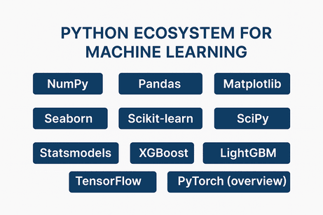
This lesson gives you a practical “map” of the main Python libraries used in Machine Learning: what each one is for, when to use it, and small code snippets you can reuse.
1) Installation (recommended)
Option A — pip (most common)
python -m pip install -U pip
pip install numpy pandas matplotlib seaborn scikit-learn scipy statsmodels xgboost lightgbm
pip install torch torchvision torchaudio
pip install tensorflow
Option B — conda (often easier for scientific stacks)
conda install -c conda-forge numpy pandas matplotlib seaborn scikit-learn scipy statsmodels xgboost lightgbm
conda install -c pytorch pytorch torchvision torchaudio
conda install -c conda-forge tensorflow
2) The “stack” in one picture
Typical workflow:
NumPy → Pandas → (Matplotlib/Seaborn) → SciPy/Statsmodels → Scikit-learn → (XGBoost/LightGBM) → (TensorFlow/PyTorch)
- Data arrays & math: NumPy
- Data tables & cleaning: Pandas
- Plots: Matplotlib + Seaborn
- Stats & scientific methods: SciPy + Statsmodels
- Classical ML: Scikit-learn
- Gradient boosting (tabular): XGBoost / LightGBM
- Deep Learning: TensorFlow / PyTorch
3) Quick comparison table
| Library | Main role | Best for | Typical output |
|---|---|---|---|
| NumPy | Fast arrays + linear algebra | Core numeric computation | ndarray |
| Pandas | Dataframes + cleaning | CSV/Excel/SQL data work | DataFrame |
| Matplotlib | Low-level plotting | Full control of plots | Figures/Axes |
| Seaborn | High-level statistical plots | Quick, pretty EDA | Matplotlib plots |
| SciPy | Scientific algorithms | Optimization, signal, stats utilities | Arrays/values |
| Statsmodels | Statistical modeling | Regression inference, p-values, ARIMA | Rich summaries |
| Scikit-learn | Classical ML toolkit | Preprocessing + models + CV | Estimators |
| XGBoost | Boosted trees (strong) | High accuracy tabular ML | Booster model |
| LightGBM | Boosted trees (fast) | Large datasets, speed/memory | Booster model |
| TensorFlow | Deep learning framework | Production pipelines, Keras training | Neural net |
| PyTorch | Deep learning framework | Research, flexibility, custom models | Neural net |
4) NumPy — arrays & linear algebra
When to use
- You need fast numeric computing (vectors/matrices).
- You’re implementing algorithms or preparing data for ML.
Demo
import numpy as np

X = np.array([[1.0, 2.0],
              [2.0, 0.5],
              [0.0, 1.0]])

w = np.array([0.4, -0.2])

# Linear model: y = Xw
y_pred = X @ w
print(y_pred)

# Basic stats
print("mean:", X.mean(axis=0))
print("std:", X.std(axis=0))
5) Pandas — data cleaning & feature prep
When to use
- Loading CSV/Excel, handling missing values, grouping, joins.
- Feature engineering on tabular data.
Demo
import pandas as pd

df = pd.DataFrame({
    "age": [22, 35, None, 41],
    "salary": [3500, 5400, 4200, 6100],
    "city": ["Rabat", "Casablanca", "Rabat", "Marrakesh"]
})

# Fix missing values
df["age"] = df["age"].fillna(df["age"].median())

# Encode a categorical feature (simple example)
df = pd.get_dummies(df, columns=["city"], drop_first=True)

print(df)
6) Matplotlib — plotting (full control)
When to use
- You want complete control over plot details.
- You’re making publication-quality figures.
Demo
import matplotlib.pyplot as plt

x = [1, 2, 3, 4]
y = [2.2, 2.9, 3.7, 4.1]

plt.plot(x, y, marker="o")
plt.title("Simple Line Plot")
plt.xlabel("x")
plt.ylabel("y")
plt.grid(True)
plt.show()
7) Seaborn — fast EDA plots (built on Matplotlib)
When to use
- Quick exploratory plots: distributions, correlations, pairplots.
- You want nice defaults with minimal code.
Demo
import seaborn as sns
import pandas as pd

tips = sns.load_dataset("tips")  # sample dataset
sns.scatterplot(data=tips, x="total_bill", y="tip", hue="time")
8) Scikit-learn — the core ML toolbox
When to use
- Classification, regression, clustering.
- Preprocessing, pipelines, cross-validation, metrics.
Demo: pipeline + train/test + metrics
from sklearn.model_selection import train_test_split
from sklearn.preprocessing import StandardScaler
from sklearn.linear_model import LogisticRegression
from sklearn.pipeline import Pipeline
from sklearn.metrics import accuracy_score
from sklearn.datasets import load_iris

X, y = load_iris(return_X_y=True)

X_train, X_test, y_train, y_test = train_test_split(
    X, y, test_size=0.2, random_state=42, stratify=y
)

model = Pipeline([
    ("scaler", StandardScaler()),
    ("clf", LogisticRegression(max_iter=200))
])

model.fit(X_train, y_train)
pred = model.predict(X_test)

print("Accuracy:", accuracy_score(y_test, pred))
9) SciPy — scientific utilities (optimization, distance, signal, stats)
When to use
- Optimization (
minimize), advanced stats, interpolation, signal processing. - You need scientific functions beyond NumPy.
Demo: optimization
import numpy as np
from scipy.optimize import minimize

def f(w):
    # simple convex function
    return (w[0]-1)**2 + (w[1]+2)**2

res = minimize(f, x0=np.array([0.0, 0.0]))
print(res.x, res.fun)
10) Statsmodels — statistics with inference (p-values, confidence intervals)
When to use
- You need interpretability and statistical tests (not just prediction).
- Econometrics, linear regression reports, time-series (ARIMA).
Demo: OLS regression summary
import numpy as np
import statsmodels.api as sm

np.random.seed(0)
X = np.random.randn(100, 2)
beta = np.array([2.0, -1.0])
y = X @ beta + np.random.randn(100) * 0.5

X_const = sm.add_constant(X)  # adds intercept
model = sm.OLS(y, X_const).fit()

print(model.summary())
11) XGBoost — powerful gradient boosting for tabular ML
When to use
- Tabular data competitions, strong baseline, handles non-linearities well.
- Works great with feature-engineered numeric/categorical encodings.
Demo (sklearn API)
from xgboost import XGBClassifier
from sklearn.datasets import load_breast_cancer
from sklearn.model_selection import train_test_split
from sklearn.metrics import roc_auc_score

X, y = load_breast_cancer(return_X_y=True)
X_train, X_test, y_train, y_test = train_test_split(X, y, test_size=0.2, random_state=42)

model = XGBClassifier(
    n_estimators=300,
    learning_rate=0.05,
    max_depth=4,
    subsample=0.9,
    colsample_bytree=0.9,
    eval_metric="logloss",
    random_state=42
)

model.fit(X_train, y_train)
proba = model.predict_proba(X_test)[:, 1]
print("AUC:", roc_auc_score(y_test, proba))
12) LightGBM — fast gradient boosting (great for large datasets)
When to use
- Very large datasets, speed/memory matters.
- Strong for tabular ML; often faster than XGBoost depending on setup.
Demo (sklearn API)
from lightgbm import LGBMClassifier
from sklearn.datasets import load_breast_cancer
from sklearn.model_selection import train_test_split
from sklearn.metrics import roc_auc_score

X, y = load_breast_cancer(return_X_y=True)
X_train, X_test, y_train, y_test = train_test_split(X, y, test_size=0.2, random_state=42)

model = LGBMClassifier(
    n_estimators=500,
    learning_rate=0.05,
    num_leaves=31,
    subsample=0.9,
    colsample_bytree=0.9,
    random_state=42
)

model.fit(X_train, y_train)
proba = model.predict_proba(X_test)[:, 1]
print("AUC:", roc_auc_score(y_test, proba))
13) TensorFlow (overview) — deep learning, often via Keras
When to use
- You want a smooth high-level API (Keras) and strong production tooling.
- Deployment ecosystems (SavedModel, TF Serving, TF Lite) are important.
Minimal Keras example
import tensorflow as tf
from tensorflow import keras

model = keras.Sequential([
    keras.layers.Dense(32, activation="relu", input_shape=(4,)),
    keras.layers.Dense(3, activation="softmax")
])

model.compile(optimizer="adam", loss="sparse_categorical_crossentropy", metrics=["accuracy"])
print(model.summary())
14) PyTorch (overview) — deep learning with maximum flexibility
When to use
- Research, custom architectures, full control of training loops.
- You want a Pythonic, “build-it-yourself” style.
Minimal example
import torch
import torch.nn as nn

model = nn.Sequential(
    nn.Linear(4, 32),
    nn.ReLU(),
    nn.Linear(32, 3)
)

x = torch.randn(5, 4)
logits = model(x)
print(logits.shape)
15) Which one should you use? (practical guide)
- Learning ML fundamentals: NumPy + Pandas + Matplotlib/Seaborn + Scikit-learn
- Statistical modeling & reports: Statsmodels (+ Pandas)
- Tabular accuracy (industry baseline): LightGBM / XGBoost
- Deep learning (vision/NLP/audio): PyTorch or TensorFlow
- Scientific computing / signals / optimization: SciPy





💬 Comments
No comments yet. Be the first to comment!
Login to comment.