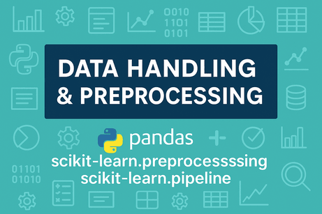
This tutorial shows a practical, repeatable workflow for preparing data for Machine Learning using pandas, sklearn.preprocessing, and sklearn.pipeline.

1) Loading datasets

A) Load a CSV with pandas

import pandas as pd

df = pd.read_csv("data.csv")  # path to your dataset
print(df.shape)
print(df.head())
print(df.dtypes)

B) Load a built-in dataset (example: California housing)

from sklearn.datasets import fetch_california_housing
import pandas as pd

data = fetch_california_housing(as_frame=True)
df = data.frame  # includes features + target column
print(df.head())

2) Cleaning data (basic checks)

Quick inspection checklist

# 1) duplicates
dup_count = df.duplicated().sum()
print("duplicates:", dup_count)

# 2) missing values
print(df.isna().sum().sort_values(ascending=False).head(10))

# 3) basic stats
print(df.describe(include="all").T.head(15))

Remove duplicates

df = df.drop_duplicates()

Fix text issues (trim spaces, normalize)

# example: cleaning a "city" column
if "city" in df.columns:
    df["city"] = df["city"].astype(str).str.strip().str.lower()

3) Handling missing values

A) Drop rows/columns (simple but risky)

# drop rows with any missing values
df_dropped = df.dropna()

# drop columns with too many missing values (example threshold: 40%)
threshold = 0.4
to_drop = [c for c in df.columns if df[c].isna().mean() > threshold]
df = df.drop(columns=to_drop)
print("dropped columns:", to_drop)

B) Impute missing values (recommended)

You’ll usually impute:

• numeric → median (robust to outliers)
• categorical → most frequent

In scikit-learn we do this inside a pipeline (best practice). You’ll see it below.

4) Encoding categorical variables

Common strategies:

• One-Hot Encoding (most common): turns categories into binary columns
• Ordinal Encoding: for ordered categories (low < medium < high)

Example (pandas one-hot for quick exploration):

df_encoded = pd.get_dummies(df, columns=["city"], drop_first=True)  # if "city" exists

Best practice for ML: use OneHotEncoder inside a pipeline (shown later).

5) Feature scaling

Why scale?

• Algorithms that use distances/gradients (KNN, SVM, Logistic Regression, Neural Nets) benefit a lot.
• Tree-based models (Decision Trees, Random Forest, XGBoost) usually don’t need scaling.

Common scalers:

• StandardScaler: mean=0, std=1 (default choice)
• MinMaxScaler: maps to [0, 1] (useful for bounded features)

We’ll use StandardScaler in the pipeline.

6) Train / validation / test split

Typical split:

• train: 70–80%
• validation: 10–15%
• test: 10–15%

A) Train/test split

from sklearn.model_selection import train_test_split

target_col = "target"  # change this
X = df.drop(columns=[target_col])
y = df[target_col]

X_train, X_test, y_train, y_test = train_test_split(
    X, y, test_size=0.2, random_state=42
)

B) Add validation split (from train)

X_train, X_val, y_train, y_val = train_test_split(
    X_train, y_train, test_size=0.25, random_state=42
)
# 0.25 of 0.8 = 0.2 => train 60%, val 20%, test 20%
print(X_train.shape, X_val.shape, X_test.shape)

Tip: For classification, use stratify=y in train_test_split to keep class proportions.

7) Pipelines (best practice)

A Pipeline chains preprocessing + model steps so you:

• avoid data leakage (scaling fitted only on train)
• keep code clean and reproducible
• can cross-validate safely

We’ll build:

• numeric preprocessing: impute median + standardize
• categorical preprocessing: impute most frequent + one-hot encode
• combine them using ColumnTransformer
• wrap everything in a Pipeline

Full example with pandas + sklearn.preprocessing + sklearn.pipeline

import pandas as pd

from sklearn.model_selection import train_test_split
from sklearn.compose import ColumnTransformer
from sklearn.pipeline import Pipeline

from sklearn.impute import SimpleImputer
from sklearn.preprocessing import OneHotEncoder, StandardScaler

from sklearn.linear_model import LogisticRegression
# For regression, swap with: from sklearn.linear_model import LinearRegression

# ---- 1) Load data ----
df = pd.read_csv("data.csv")  # replace with your path

target_col = "target"         # replace with your target column name
X = df.drop(columns=[target_col])
y = df[target_col]

# ---- 2) Split data ----
X_train, X_test, y_train, y_test = train_test_split(
    X, y, test_size=0.2, random_state=42
)

# ---- 3) Detect column types ----
numeric_features = X_train.select_dtypes(include=["number"]).columns
categorical_features = X_train.select_dtypes(exclude=["number"]).columns

# ---- 4) Build preprocessors ----
numeric_transformer = Pipeline(steps=[
    ("imputer", SimpleImputer(strategy="median")),
    ("scaler", StandardScaler()),
])

categorical_transformer = Pipeline(steps=[
    ("imputer", SimpleImputer(strategy="most_frequent")),
    ("onehot", OneHotEncoder(handle_unknown="ignore")),
])

preprocessor = ColumnTransformer(
    transformers=[
        ("num", numeric_transformer, numeric_features),
        ("cat", categorical_transformer, categorical_features),
    ]
)

# ---- 5) Build full pipeline (preprocess + model) ----
model = LogisticRegression(max_iter=1000)

clf = Pipeline(steps=[
    ("preprocess", preprocessor),
    ("model", model)
])

# ---- 6) Fit ----
clf.fit(X_train, y_train)

# ---- 7) Evaluate ----
print("Train score:", clf.score(X_train, y_train))
print("Test score:", clf.score(X_test, y_test))

Why this pipeline is “correct”

• Missing values are handled inside the pipeline.
• One-hot encoding is learned from training data and applied consistently to test data.
• Scaling is fitted only on training data (no leakage).

8) A compact “preprocessing-only” pipeline (transform features)

Sometimes you want to just transform X:

X_train_ready = preprocessor.fit_transform(X_train)
X_test_ready = preprocessor.transform(X_test)

print(type(X_train_ready), X_train_ready.shape)

9) Common preprocessing mistakes to avoid

• Fitting scalers/encoders on the full dataset before splitting → leakage.
• Using pandas get_dummies separately on train and test → mismatched columns.
• Dropping all missing rows blindly → you may delete most of your data.
• Scaling target variable without a reason (only for specific models/metrics).