0. Introduction
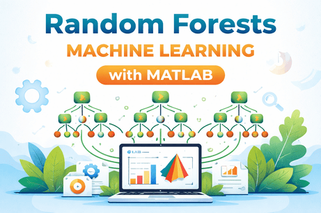
Random Forests are ensemble learning methods built from many decision trees. Instead of relying on a single tree, a random forest combines the predictions of many trees to improve stability and generalization. In MATLAB, the two main command-line paths are TreeBagger and bagged tree ensembles via fitcensemble or fitrensemble. MathWorks explicitly describes TreeBagger as an ensemble of bagged decision trees for classification or regression, and it notes that fitcensemble/fitrensemble can also grow bagged tree ensembles and random forests.
This tutorial explains what random forests are, how they work, when to use them, and how to implement them in MATLAB for both classification and regression. It also shows how random forests relate to bagging, feature randomness, out-of-bag error, feature importance, and the Classification Learner / Regression Learner apps.
1. What is a Random Forest?
A random forest is an ensemble of decision trees trained on bootstrap samples of the data. In addition, when a tree is grown, the algorithm considers only a random subset of predictors at each split, which increases diversity among trees. MATLAB’s TreeBagger documentation describes bagging as bootstrap aggregation and explains that bagging reduces overfitting and improves generalization; MathWorks also states that fitcensemble with method "Bag" uses bagging with random predictor selections at each split by default, which is the random forest behavior.
In simple terms:
- build many decision trees,
- train each tree on a slightly different sample of the data,
- use random subsets of predictors during splitting,
- combine the trees’ predictions.
For classification, the forest usually predicts by majority vote. For regression, it averages the tree predictions. This is consistent with MATLAB’s bagged classification and regression ensemble workflows.
2. Why use Random Forests?
Random forests are popular because they are:
- more robust than a single decision tree,
- able to model nonlinear relationships,
- useful for both classification and regression,
- often strong baseline and production models,
- capable of estimating predictor importance.
MathWorks positions random forests as tree ensembles created through bagging, and its random-forest-related examples include predictor importance and hyperparameter tuning workflows for regression forests.
3. Main ideas behind Random Forests
3.1 Bagging
Bagging means bootstrap aggregation. Each tree is trained on a bootstrap sample drawn from the training data. MathWorks defines TreeBagger as a bagged decision-tree ensemble and notes that bagging reduces overfitting effects from individual trees.
3.2 Random predictor selection
Random forests do not test all predictors at every split. They test only a random subset, which makes trees less correlated and often improves ensemble performance. MathWorks explicitly states that fitcensemble with "Bag" uses random predictor selections at each split by default.
3.3 Ensemble voting or averaging
For classification, multiple trees vote for a class. For regression, the predictions are averaged. That is the standard behavior of bagged ensembles in MATLAB classification and regression workflows.
3.4 Out-of-bag validation
Because each tree sees only a bootstrap sample, some training observations are left out for that tree. These are called out-of-bag observations and can be used to estimate generalization performance without a separate validation set. TreeBagger supports out-of-bag prediction error and related analysis.
3.5 Predictor importance
Random forests can estimate which predictors matter most. MathWorks has dedicated examples on selecting predictors for random forests and supports importance-style analyses in tree-bagging workflows.
4. MATLAB tools you need to know
The most important MATLAB tools for random forests are:
TreeBagger→ bagged decision-tree ensembles for classification or regression,fitcensemble→ classification ensembles, including bagged trees / random forests,fitrensemble→ regression ensembles, including bagged trees / random forests,predict→ predictions for new data,- Classification Learner → app workflow for bagged tree classifiers,
- Regression Learner → app workflow for bagged tree regressors.
MathWorks states that fitcensemble can boost or bag classification trees or grow a random forest, and that fitrensemble can bag regression trees or grow a random forest.
Part I — Random Forest Classification with TreeBagger
5. First simple example
Let us begin with a small binary classification dataset.
clc;
clear;
close all;

% Example data
X = [1 2;
     2 3;
     2 1;
     3 2;
     6 7;
     7 8;
     8 7;
     7 6];

Y = categorical([1; 1; 1; 1; 2; 2; 2; 2]);

% Train random forest classifier
Mdl = TreeBagger(50, X, Y, ...
    'Method', 'classification', ...
    'OOBPrediction', 'On');

% Predict on training data
[YPred, scores] = predict(Mdl, X);

disp('Predicted labels:');
disp(YPred);

disp('Scores:');
disp(scores);
TreeBagger creates an ensemble of bagged decision trees for classification or regression. For classification, predictions returned by predict are often strings or categorical-like labels depending on how the response is stored, so you may need to convert them before computing accuracy.
6. Visualizing out-of-bag classification error
A useful feature of TreeBagger is out-of-bag error tracking.
clc;
clear;
close all;

X = [1 2;
     2 3;
     2 1;
     3 2;
     6 7;
     7 8;
     8 7;
     7 6];

Y = categorical([1;1;1;1;2;2;2;2]);

Mdl = TreeBagger(100, X, Y, ...
    'Method', 'classification', ...
    'OOBPrediction', 'On');

oobErrorBaggedEnsemble = oobError(Mdl);

plot(oobErrorBaggedEnsemble, 'LineWidth', 1.5);
xlabel('Number of Grown Trees');
ylabel('Out-of-Bag Classification Error');
title('OOB Error for Random Forest Classification');
grid on;
This plot helps you see whether adding more trees improves performance or whether the error stabilizes. The TreeBagger workflow supports out-of-bag diagnostics like this directly.
7. Train/test split for classification
Although out-of-bag estimates are useful, a separate test set is still a good habit.
clc;
clear;
close all;

% Dataset
X = [1 2;
     2 3;
     2 1;
     3 2;
     6 7;
     7 8;
     8 7;
     7 6;
     1.5 2.5;
     6.5 7.5];

Y = categorical([1;1;1;1;2;2;2;2;1;2]);

% Holdout split
rng(1);
cv = cvpartition(Y, 'HoldOut', 0.3);

XTrain = X(training(cv), :);
YTrain = Y(training(cv), :);

XTest = X(test(cv), :);
YTest = Y(test(cv), :);

% Train random forest
Mdl = TreeBagger(100, XTrain, YTrain, ...
    'Method', 'classification', ...
    'OOBPrediction', 'On');

% Predict on test data
YPred = predict(Mdl, XTest);
YPred = categorical(YPred);

% Accuracy
accuracy = mean(YPred == YTest) * 100;
fprintf('Test Accuracy = %.2f%%\n', accuracy);
This is a practical workflow for small and medium datasets.
8. Confusion matrix
For classification, a confusion matrix is very useful.
cm = confusionmat(YTest, YPred);
disp('Confusion Matrix:');
disp(cm);

confusionchart(YTest, YPred);
title('Random Forest Confusion Matrix');
This lets you inspect misclassifications, not only overall accuracy.
9. Multiclass classification with iris
Random forests handle multiclass classification naturally.
clc;
clear;
close all;

load fisheriris

X = meas;
Y = categorical(species);

% Train random forest
Mdl = TreeBagger(100, X, Y, ...
    'Method', 'classification', ...
    'OOBPrediction', 'On');

% Predict
YPred = predict(Mdl, X);
YPred = categorical(YPred);

% Accuracy
accuracy = mean(YPred == Y) * 100;
fprintf('Training Accuracy = %.2f%%\n', accuracy);

confusionchart(Y, YPred);
title('Random Forest on Fisher Iris');
Since TreeBagger is a classification or regression ensemble of trees, it works well for multiclass classification problems as well.
Part II — Random Forest Classification with fitcensemble
10. Why use fitcensemble?
MATLAB also supports random-forest-style classification through fitcensemble. MathWorks explicitly states that when Method is "Bag", fitcensemble uses bagging with random predictor selections at each split by default.
clc;
clear;
close all;

load fisheriris

X = meas;
Y = species;

% Random-forest-style bagged tree ensemble
Mdl = fitcensemble(X, Y, ...
    'Method', 'Bag', ...
    'NumLearningCycles', 100);

YPred = predict(Mdl, X);

accuracy = mean(strcmp(YPred, Y)) * 100;
fprintf('Training Accuracy = %.2f%%\n', accuracy);
This is often a nice command-line alternative when you want to stay inside the ensemble framework.
11. Classification loss with fitcensemble
clc;
clear;
close all;

load fisheriris

X = meas;
Y = species;

Mdl = fitcensemble(X, Y, ...
    'Method', 'Bag', ...
    'NumLearningCycles', 100);

L = loss(Mdl, X, Y);

fprintf('Classification Loss = %.4f\n', L);
fprintf('Approximate Accuracy = %.2f%%\n', (1 - L) * 100);
MathWorks documents classification ensemble objects for bagging and random-forest-style workflows, and loss is a standard way to evaluate such models.
Part III — Random Forest Regression
12. Random forest regression with TreeBagger
Random forests are also very effective for regression.
clc;
clear;
close all;

% Simple regression data
X = (1:10)';
Y = [1.2; 1.9; 2.8; 3.9; 5.1; 5.9; 7.0; 8.1; 8.9; 10.2];

% Train random forest regressor
Mdl = TreeBagger(100, X, Y, ...
    'Method', 'regression', ...
    'OOBPrediction', 'On');

% Predict
YPred = predict(Mdl, X);

disp(table(X, Y, YPred));
MathWorks documents TreeBagger for both classification and regression.
13. Plotting random forest regression predictions
clc;
clear;
close all;

X = (1:10)';
Y = [1.2; 1.9; 2.8; 3.9; 5.1; 5.9; 7.0; 8.1; 8.9; 10.2];

Mdl = TreeBagger(100, X, Y, ...
    'Method', 'regression', ...
    'OOBPrediction', 'On');

YPred = predict(Mdl, X);

plot(X, Y, 'o', 'MarkerSize', 8, 'LineWidth', 1.5);
hold on;
plot(X, YPred, '-s', 'LineWidth', 1.5);
xlabel('X');
ylabel('Y');
title('Random Forest Regression');
legend('Original Data', 'Predictions');
grid on;
This gives a simple visual comparison between real and predicted values.
14. Regression metrics: MAE, MSE, RMSE
clc;
clear;
close all;

X = (1:10)';
Y = [1.2; 1.9; 2.8; 3.9; 5.1; 5.9; 7.0; 8.1; 8.9; 10.2];

Mdl = TreeBagger(100, X, Y, 'Method', 'regression');
YPred = predict(Mdl, X);

MAE = mean(abs(Y - YPred));
MSE = mean((Y - YPred).^2);
RMSE = sqrt(MSE);

fprintf('MAE  = %.4f\n', MAE);
fprintf('MSE  = %.4f\n', MSE);
fprintf('RMSE = %.4f\n', RMSE);
For regression, these metrics are usually more informative than a simple visual check.
15. Random forest regression with fitrensemble
MathWorks states that to bag regression trees or grow a random forest, you can use fitrensemble or TreeBagger.
clc;
clear;
close all;

load carsmall

tbl = table(Horsepower, Weight, MPG);
tbl = rmmissing(tbl);

Mdl = fitrensemble(tbl, 'MPG ~ Horsepower + Weight', ...
    'Method', 'Bag', ...
    'NumLearningCycles', 100);

YPred = predict(Mdl, tbl(:, {'Horsepower','Weight'}));

RMSE = sqrt(mean((tbl.MPG - YPred).^2));
fprintf('RMSE = %.4f\n', RMSE);

plot(tbl.MPG, YPred, 'o');
xlabel('Actual MPG');
ylabel('Predicted MPG');
title('Random Forest Regression with fitrensemble');
grid on;
This is a clean formula-based regression forest workflow.
Part IV — Out-of-Bag Error and Predictor Importance
16. Why out-of-bag error matters
Out-of-bag error is one of the conveniences of random forests. Because each tree leaves out some training observations, those unused observations can serve as a built-in validation sample for that tree. TreeBagger supports OOB prediction and OOB error monitoring directly.
For classification:
clc;
clear;
close all;

load fisheriris

Mdl = TreeBagger(150, meas, species, ...
    'Method', 'classification', ...
    'OOBPrediction', 'On');

figure;
plot(oobError(Mdl), 'LineWidth', 1.5);
xlabel('Number of Trees');
ylabel('Out-of-Bag Error');
title('OOB Error for Classification Forest');
grid on;

For regression:

clc;
clear;
close all;

load carsmall

tbl = table(Horsepower, Weight, MPG);
tbl = rmmissing(tbl);

X = tbl{:, {'Horsepower','Weight'}};
Y = tbl.MPG;

Mdl = TreeBagger(150, X, Y, ...
    'Method', 'regression', ...
    'OOBPrediction', 'On');

figure;
plot(oobError(Mdl), 'LineWidth', 1.5);
xlabel('Number of Trees');
ylabel('Out-of-Bag Mean Squared Error');
title('OOB Error for Regression Forest');
grid on;
17. Predictor importance
Random forests are often used to estimate which variables contribute most to prediction. MathWorks has an example specifically about selecting predictors for random forests, which reflects the importance-analysis role forests can play.
With TreeBagger, a common workflow is:
clc;
clear;
close all;

load fisheriris

Mdl = TreeBagger(100, meas, species, ...
    'Method', 'classification', ...
    'OOBPredictorImportance', 'On');

bar(Mdl.OOBPermutedPredictorDeltaError);
xlabel('Predictor Index');
ylabel('Importance');
title('OOB Permuted Predictor Importance');
grid on;
This gives an importance score for each predictor based on how much prediction error increases when that predictor is permuted.
Part V — Hyperparameters and Practical Choices
18. Important hyperparameters
The main choices in a random forest include:
- number of trees,
- tree depth or tree size,
- number of predictors sampled at each split,
- minimum leaf size.
MathWorks’ random-forest-related examples and ensemble documentation emphasize these kinds of model controls, including predictor-selection techniques and Bayesian tuning examples for regression forests.
A practical rule
- Start with 100 trees.
- Increase the number of trees until OOB error stabilizes.
- Use OOB error or a validation set to compare settings.
- Do not rely only on training accuracy.
19. More trees vs better trees
Adding more trees usually improves stability, but after some point the gain becomes small. OOB error plots are useful for deciding when you have enough trees. That is one reason the TreeBagger workflow is convenient.
Part VI — Classification Learner and Regression Learner
20. Classification Learner
MATLAB’s Classification Learner app includes bagged trees, and MathWorks indicates that bagged trees there correspond to a random forest ensemble method.
Open it with:
classificationLearnerTypical workflow:
- import your dataset,
- choose the response variable,
- select Bagged Trees,
- train the model,
- compare validation results,
- export the model or generated code.
21. Regression Learner
For regression, Regression Learner supports ensemble workflows including bagged trees / random-forest-style regressors through MATLAB’s regression ensemble infrastructure. MathWorks documents regression tree ensembles and app-based regression exploration.
Open it with:
regressionLearnerTypical workflow:
- import the data,
- choose the numeric target,
- train a bagged tree ensemble,
- compare results,
- export the trained model.
<hr>
Part VII — End-to-End Mini Projects
22. Classification project: predict pass or fail
clc;
clear;
close all;

% Example student data
StudyHours = [1;2;2;3;4;5;5;6;7;8];
Attendance = [50;55;60;65;70;75;80;85;90;95];
Pass = categorical([0;0;0;0;0;1;1;1;1;1]);

X = [StudyHours Attendance];
Y = Pass;

% Train/test split
rng(2);
cv = cvpartition(Y, 'HoldOut', 0.3);

XTrain = X(training(cv), :);
YTrain = Y(training(cv), :);

XTest = X(test(cv), :);
YTest = Y(test(cv), :);

% Train random forest classifier
Mdl = TreeBagger(100, XTrain, YTrain, ...
    'Method', 'classification', ...
    'OOBPrediction', 'On');

% Predict
YPred = predict(Mdl, XTest);
YPred = categorical(YPred);

% Accuracy
accuracy = mean(YPred == YTest) * 100;
fprintf('Test Accuracy = %.2f%%\n', accuracy);

% Confusion matrix
confusionchart(YTest, YPred);
title('Pass/Fail Random Forest');

% Predict a new student
newStudent = [6 82];
newClass = predict(Mdl, newStudent);

disp('Predicted class for new student:');
disp(newClass);
This project includes train/test split, ensemble training, evaluation, and prediction for a new observation.
23. Regression project: predict house prices
clc;
clear;
close all;

% Example house dataset
Size = [50; 60; 70; 80; 90; 100; 110; 120];
Rooms = [2; 3; 3; 4; 4; 5; 5; 6];
Age = [20; 18; 15; 12; 10; 8; 5; 3];
Price = [100; 120; 135; 150; 170; 190; 210; 230];

X = [Size Rooms Age];
Y = Price;

% Train/test split
rng(3);
idx = randperm(length(Y));

trainIdx = idx(1:6);
testIdx = idx(7:8);

XTrain = X(trainIdx, :);
YTrain = Y(trainIdx);

XTest = X(testIdx, :);
YTest = Y(testIdx);

% Train regression forest
Mdl = TreeBagger(100, XTrain, YTrain, ...
    'Method', 'regression', ...
    'OOBPrediction', 'On');

% Predict
YPred = predict(Mdl, XTest);

% RMSE
RMSE = sqrt(mean((YTest - YPred).^2));
fprintf('Test RMSE = %.4f\n', RMSE);

disp(table(YTest, YPred, 'VariableNames', {'ActualPrice','PredictedPrice'}));
This is a simple end-to-end regression forest workflow.
Part VIII — Common mistakes beginners make
24. Confusing a single tree with a forest
A random forest is not one tree. It is a bagged ensemble of many trees, often with random predictor selection at each split. MATLAB distinguishes single-tree functions (fitctree, fitrtree) from forest-like ensemble tools (TreeBagger, fitcensemble, fitrensemble).
25. Using too few trees
Very small forests can be unstable. It is usually better to start with dozens or hundreds of trees and use OOB error to see whether performance has stabilized.
26. Looking only at training accuracy
A forest can still overfit or give an overly optimistic picture on the training set. OOB error or a holdout test set gives a more useful estimate.
27. Ignoring predictor importance carefully
Importance scores are useful, but they are not the same as causal effects. Treat them as model-based importance, not proof of cause.
28. Using the wrong MATLAB function for the task
Use:
TreeBaggerfor bagged tree ensembles in classification or regression,fitcensemblefor classification ensembles,fitrensemblefor regression ensembles. MathWorks explicitly documents these pathways.
Part IX — When should you use Random Forests?
Random forests are a good choice when:
- you want strong performance with relatively little feature engineering,
- relationships may be nonlinear,
- interactions may be complex,
- you want built-in importance estimates,
- you need both classification and regression options.
You may avoid them when:
- model interpretability at the exact equation level is essential,
- memory or prediction speed is extremely constrained,
- your dataset is so simple that a smaller model is enough.
These are practical implications of how bagged tree ensembles work and how MATLAB represents them.
Part X — Summary
Random forests are among the most useful general-purpose machine learning methods. In MATLAB, you can build them with TreeBagger, or through bagged ensemble workflows using fitcensemble and fitrensemble. MATLAB also supports random-forest-style models in Classification Learner and Regression Learner. Out-of-bag error, predictor importance, multiclass classification, and regression workflows are all part of the MATLAB ecosystem for forests.
A strong practical workflow is:
- prepare the data,
- choose classification or regression,
- train a forest with enough trees,
- inspect OOB error,
- evaluate on unseen data,
- inspect predictor importance when useful,
- deploy the best model.
Part XI — MATLAB cheat sheet
Classification with TreeBagger
Mdl = TreeBagger(100, X, Y, 'Method', 'classification', 'OOBPrediction', 'On');
YPred = predict(Mdl, Xnew);
Regression with TreeBagger
Mdl = TreeBagger(100, X, Y, 'Method', 'regression', 'OOBPrediction', 'On');
YPred = predict(Mdl, Xnew);
Classification with fitcensemble
Mdl = fitcensemble(X, Y, 'Method', 'Bag', 'NumLearningCycles', 100);
YPred = predict(Mdl, Xnew);
Regression with fitrensemble
Mdl = fitrensemble(X, Y, 'Method', 'Bag', 'NumLearningCycles', 100);
YPred = predict(Mdl, Xnew);
OOB error
plot(oobError(Mdl));Predictor importance
Mdl = TreeBagger(100, X, Y, 'Method', 'classification', 'OOBPredictorImportance', 'On');
bar(Mdl.OOBPermutedPredictorDeltaError);
These workflows match MATLAB’s documented random-forest / bagged-tree ensemble ecosystem.
Practice exercises
Solution of Exercise 1
Train a random forest classifier on a small binary dataset and compute test accuracy
Solution of Exercise 2
Use the fisheriris dataset to build a multiclass random forest classifier
Solution of Exercise 3
Plot the out-of-bag classification error as the number of trees grows
Solution of Exercise 4
Train a random forest regressor on a simple numeric dataset and compute RMSE
Solution of Exercise 5
Build a small end-to-end random forest project with train/test split, evaluation, and prediction for a new observation
Short recap
Exercise 1
Train a binary random forest classifier and compute test accuracy.
Exercise 2
Build a multiclass random forest classifier with the iris dataset.
Exercise 3
Plot out-of-bag classification error.
Exercise 4
Train a random forest regressor and compute RMSE.
Exercise 5
Create a full random forest mini-project with training, testing, evaluation, and prediction.









💬 Comments
No comments yet. Be the first to comment!
Login to comment.