0. Introdution
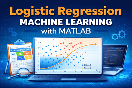
Logistic Regression is one of the most important supervised machine learning algorithms for classification. Unlike linear regression, which predicts continuous values, logistic regression predicts the probability of belonging to a class, then converts that probability into a class label. In MATLAB, a common documented path for binary GLM logistic regression is fitglm, while efficiently trained logistic regression in Classification Learner uses fitclinear for binary data and fitcecoc for multiclass data. MATLAB also provides the Classification Learner app for GUI-based workflows.
This tutorial explains what logistic regression is, when to use it, how it works conceptually, and how to implement it in MATLAB with practical examples for binary and multiclass classification. The MATLAB-specific parts below are aligned with current MathWorks documentation on fitglm, Classification Learner, and classifier options.
1. What is Logistic Regression?
Logistic Regression is a supervised learning algorithm used mainly for classification problems. It models class probabilities from a linear combination of predictors, and in MATLAB’s Classification Learner, logistic regression classifiers are described as modeling class probabilities as a function of that linear combination. Binary GLM logistic regression there is based on fitglm.
In simple terms:
- Binary logistic regression predicts one of two classes, such as yes/no or spam/not spam.
- Multiclass logistic regression predicts one of several classes.
- The model outputs a probability, then assigns the most likely class. MathWorks’ documentation and examples for Classification Learner describe binary GLM logistic regression as a classifier type and note that the app reports validation accuracy after training.
2. Why use Logistic Regression?
Logistic Regression is popular because it is:
- simple,
- interpretable,
- fast,
- strong as a baseline classifier,
- effective for many binary classification tasks.
MathWorks specifically describes logistic regression as a popular classifier to try because it is easy to interpret. It also distinguishes standard binary GLM logistic regression from more efficient logistic regression options for larger datasets.
It is especially useful when:
- the target variable is categorical,
- you want class probabilities,
- you want a model that is easier to explain than more complex classifiers,
- you need a baseline before trying more advanced models.
3. Main concepts behind Logistic Regression
3.1 Probability output
Instead of predicting a raw numeric value like linear regression, logistic regression predicts a probability between 0 and 1 for a class. MATLAB’s logistic regression workflows are built around class probability modeling.
3.2 Decision boundary
A probability is converted into a label using a threshold. In common binary classification practice that is often 0.5, and in Classification Learner the predicted class is assigned according to the class probabilities. This means logistic regression produces a classification boundary in predictor space.
3.3 Linear combination of predictors
Like linear regression, logistic regression starts from a weighted sum of predictors:
$z = b_0 + b_1x_1 + b_2x_2 + \dots + b_nx_n$
Then it passes this through a logistic transformation to convert it into a probability.
3.4 Logit link
In MATLAB, fitglm creates a generalized linear model, and logistic regression is one of the supported GLM families. The typical binary logistic regression setup uses a binomial distribution and logit link. This is part of the fitglm workflow documented by MathWorks.
4. MATLAB tools you need to know
For logistic regression in MATLAB, the most useful tools are:
fitglm→ binary GLM logistic regression,predict→ predicted probabilities or fitted responses from the model,fitclinear→ efficient logistic regression for binary classification in larger problems,fitcecoc→ multiclass classification using binary learners,Classification Learner→ GUI-based classification workflow.
MathWorks’ classifier options page explicitly states that binary GLM logistic regression in Classification Learner uses fitglm, and efficient logistic regression uses fitclinear for binary data and fitcecoc for multiclass data.
Part I — Binary Logistic Regression in MATLAB
5. First simple example
Let us begin with a small binary classification example.
clc;
clear;
close all;

% Example data
X = [1; 2; 3; 4; 5; 6; 7; 8];
Y = [0; 0; 0; 0; 1; 1; 1; 1];

% Fit logistic regression model
mdl = fitglm(X, Y, 'Distribution', 'binomial');

% Display model
disp(mdl);
This code fits a binary generalized linear model using fitglm with a binomial distribution, which is the standard MATLAB route for GLM logistic regression. fitglm(X,y) returns a generalized linear regression model fit to predictors X and response y, and extra options can be specified through model settings.
6. Predicting probabilities
A major strength of logistic regression is that it predicts probabilities, not only labels.
clc;
clear;
close all;

X = [1; 2; 3; 4; 5; 6; 7; 8];
Y = [0; 0; 0; 0; 1; 1; 1; 1];

mdl = fitglm(X, Y, 'Distribution', 'binomial');

% Predicted probabilities
p = predict(mdl, X);

disp('Predicted probabilities:');
disp(p);
With logistic regression, the output of predict is interpreted as the model’s fitted response, which for binomial logistic regression is the estimated probability of the positive class. This fits with how MathWorks describes logistic classifiers as modeling class probabilities.
7. Converting probabilities into class labels
To turn probabilities into final class predictions, we compare them to a threshold.
clc;
clear;
close all;

X = [1; 2; 3; 4; 5; 6; 7; 8];
Y = [0; 0; 0; 0; 1; 1; 1; 1];

mdl = fitglm(X, Y, 'Distribution', 'binomial');

p = predict(mdl, X);

% Convert probabilities to labels
YPred = double(p >= 0.5);

disp(table(X, Y, p, YPred));
This shows the typical idea of logistic classification: estimate the class probability and then map it to a label. In MATLAB app-based workflows, the class with the larger assigned probability is selected as the predicted class.
8. Plotting the logistic curve
A useful visualization for one predictor is the S-shaped probability curve.
clc;
clear;
close all;

X = [1; 2; 3; 4; 5; 6; 7; 8];
Y = [0; 0; 0; 0; 1; 1; 1; 1];

mdl = fitglm(X, Y, 'Distribution', 'binomial');

xFine = linspace(min(X), max(X), 100)';
pFine = predict(mdl, xFine);

plot(X, Y, 'o');
hold on;
plot(xFine, pFine, '-', 'LineWidth', 2);
xlabel('X');
ylabel('Probability / Class');
title('Logistic Regression Curve');
legend('Training Data', 'Predicted Probability');
grid on;
This graph helps you see how the predicted probability changes as the predictor increases. It is one of the clearest ways to understand logistic regression with a single feature.
9. Binary classification example with train/test split
In machine learning, we should evaluate the model on unseen data.
clc;
clear;
close all;

% Example dataset
X = [1; 2; 3; 4; 5; 6; 7; 8; 2.5; 6.5];
Y = [0; 0; 0; 0; 1; 1; 1; 1; 0; 1];

% Random split
rng(1);
idx = randperm(length(X));

trainIdx = idx(1:7);
testIdx  = idx(8:end);

XTrain = X(trainIdx);
YTrain = Y(trainIdx);

XTest = X(testIdx);
YTest = Y(testIdx);

% Train model
mdl = fitglm(XTrain, YTrain, 'Distribution', 'binomial');

% Predict probabilities
pTest = predict(mdl, XTest);

% Convert to labels
YPred = double(pTest >= 0.5);

% Accuracy
accuracy = mean(YPred == YTest) * 100;
fprintf('Test Accuracy = %.2f%%\n', accuracy);

disp(table(XTest, YTest, pTest, YPred));
This basic workflow mirrors what MATLAB’s Classification Learner also automates: import data, choose validation, train the model, and evaluate validation performance. The app’s default validation scheme is 5-fold cross-validation.
10. Confusion matrix
A confusion matrix shows the number of correct and incorrect predictions.
clc;
clear;
close all;

X = [1; 2; 3; 4; 5; 6; 7; 8; 2.5; 6.5];
Y = [0; 0; 0; 0; 1; 1; 1; 1; 0; 1];

mdl = fitglm(X, Y, 'Distribution', 'binomial');

p = predict(mdl, X);
YPred = double(p >= 0.5);

cm = confusionmat(Y, YPred);
disp('Confusion Matrix:');
disp(cm);

confusionchart(Y, YPred);
title('Confusion Matrix');
Confusion matrices are a standard way to evaluate classification models, especially when raw accuracy is not enough.
<hr>Part II — Logistic Regression with Multiple Predictors
11. Why use multiple predictors?
Real classification tasks usually depend on more than one variable. For example, predicting whether a patient has a condition might depend on age, weight, blood pressure, and other features.
12. Example with two predictors
clc;
clear;
close all;

% Two predictors
X1 = [1;2;3;4;5;6;7;8];
X2 = [8;7;6;5;4;3;2;1];

% Response
Y = [0;0;0;0;1;1;1;1];

% Build table
tbl = table(X1, X2, Y);

% Fit logistic regression
mdl = fitglm(tbl, 'Y ~ X1 + X2', 'Distribution', 'binomial');

disp(mdl);
MathWorks documents formula-based modeling with fitglm, including table workflows where you can specify predictors and response using model formulas.
13. Predicting from multiple predictors
clc;
clear;
close all;

X1 = [1;2;3;4;5;6;7;8];
X2 = [8;7;6;5;4;3;2;1];
Y  = [0;0;0;0;1;1;1;1];

tbl = table(X1, X2, Y);

mdl = fitglm(tbl, 'Y ~ X1 + X2', 'Distribution', 'binomial');

newData = table([2;6], [7;3], 'VariableNames', {'X1','X2'});
pNew = predict(mdl, newData);
YPredNew = double(pNew >= 0.5);

disp(table(newData.X1, newData.X2, pNew, YPredNew, ...
    'VariableNames', {'X1','X2','Probability','PredictedClass'}));
This is the practical prediction workflow you would use after training a binary logistic regression model.
Part III — Realistic Binary Classification Example
14. Example inspired by MATLAB’s patients data workflow
MathWorks provides an example showing Classification Learner with the patients dataset for binary GLM logistic regression. The example uses predictors like Age, Diastolic, Height, Systolic, and Weight, and response Gender.
Below is a code-based version:
clc;
clear;
close all;

load patients

% Predictors
tbl = table(Age, Diastolic, Height, Systolic, Weight, Gender);

% Remove missing values if needed
tbl = rmmissing(tbl);

% Fit binary logistic regression
mdl = fitglm(tbl, 'Gender ~ Age + Diastolic + Height + Systolic + Weight', ...
    'Distribution', 'binomial');

disp(mdl);

% Predicted probabilities
p = predict(mdl, tbl);

% Convert probabilities into class labels
% Depending on class coding, inspect probabilities first in practice
YPred = strings(height(tbl),1);
YPred(p >= 0.5) = string(unique(tbl.Gender)(2));
YPred(p < 0.5)  = string(unique(tbl.Gender)(1));

disp('First few predicted probabilities:');
disp(p(1:10));
This example is mainly pedagogical. In real practice, when the response is categorical text labels, you should verify how MATLAB encodes the response internally before manually assigning labels from probabilities.
Part IV — Evaluating Logistic Regression Models
15. Accuracy
Accuracy is the percentage of correctly classified examples.
clc;
clear;
close all;

X = [1; 2; 3; 4; 5; 6; 7; 8; 2.5; 6.5];
Y = [0; 0; 0; 0; 1; 1; 1; 1; 0; 1];

mdl = fitglm(X, Y, 'Distribution', 'binomial');

p = predict(mdl, X);
YPred = double(p >= 0.5);

accuracy = mean(YPred == Y) * 100;
fprintf('Accuracy = %.2f%%\n', accuracy);
Accuracy is easy to understand, but it can be misleading when classes are imbalanced.
16. Precision, recall, and F1-score
For many classification tasks, especially imbalanced ones, accuracy is not enough. MATLAB’s recent Classification Learner metrics include precision, recall, and F1 score among model performance metrics in the app.
You can compute them manually:
clc;
clear;
close all;

X = [1; 2; 3; 4; 5; 6; 7; 8; 2.5; 6.5];
Y = [0; 0; 0; 0; 1; 1; 1; 1; 0; 1];

mdl = fitglm(X, Y, 'Distribution', 'binomial');

p = predict(mdl, X);
YPred = double(p >= 0.5);

TP = sum((Y == 1) & (YPred == 1));
TN = sum((Y == 0) & (YPred == 0));
FP = sum((Y == 0) & (YPred == 1));
FN = sum((Y == 1) & (YPred == 0));

precision = TP / (TP + FP);
recall    = TP / (TP + FN);
f1        = 2 * (precision * recall) / (precision + recall);

fprintf('Precision = %.4f\n', precision);
fprintf('Recall    = %.4f\n', recall);
fprintf('F1-score  = %.4f\n', f1);
These metrics often tell a more useful story than accuracy alone.
Part V — Efficient Logistic Regression in MATLAB
17. When to use fitclinear
MathWorks distinguishes standard binary GLM logistic regression from efficient logistic regression. According to the classifier options page, efficient logistic regression uses fitclinear for binary class data and is recommended when you have many predictors or many observations, trading some accuracy for faster training.
Example:
clc;
clear;
close all;

% Example matrix predictors
X = [1 5;
     2 4;
     3 3;
     4 2;
     5 1;
     6 2;
     7 3;
     8 4];

Y = [0;0;0;0;1;1;1;1];

% Efficient logistic regression
mdl = fitclinear(X, Y, ...
    'Learner', 'logistic', ...
    'Regularization', 'ridge');

[label, score] = predict(mdl, X);

disp('Predicted labels:');
disp(label);

disp('Scores:');
disp(score);
This is a good option when scaling up beyond small demonstration datasets.
Part VI — Multiclass Logistic Regression in MATLAB
18. Can logistic regression handle more than two classes?
Yes, but multiclass classification is handled differently from simple binary logistic regression. In MATLAB’s classifier options, efficient logistic regression for multiclass data uses fitcecoc.
A simple practical way is to use fitcecoc with linear learners:
clc;
clear;
close all;

load fisheriris

X = meas;
Y = species;

% Multiclass linear classification via ECOC
t = templateLinear('Learner', 'logistic');

Mdl = fitcecoc(X, Y, 'Learners', t);

YPred = predict(Mdl, X);

accuracy = mean(strcmp(YPred, Y)) * 100;
fprintf('Training Accuracy = %.2f%%\n', accuracy);

confusionchart(Y, YPred);
title('Multiclass Logistic-Style ECOC Classification');
This is a practical multiclass workflow in MATLAB when you want a linear classifier with logistic-style learners.
Part VII — Using Classification Learner
19. App-based workflow
MATLAB’s Classification Learner app lets you import data, choose predictors and response, set validation schemes, train logistic regression classifiers, compare models, assess results, and investigate predictor contributions.
Open it with:
classificationLearnerTypical steps:
- import the dataset,
- choose the response variable,
- select logistic regression under classifier models,
- train the model,
- inspect validation accuracy and other metrics,
- export the trained model or generated code.
MathWorks’ example explicitly shows training a binary GLM logistic regression model in Classification Learner, with 5-fold cross-validation as the default validation choice.
Part VIII — End-to-End Mini Project
20. Project: Predict pass or fail
Here is a small complete project.
clc;
clear;
close all;

% Example student data
StudyHours = [1;2;2;3;4;5;5;6;7;8];
Attendance = [50;55;60;65;70;75;80;85;90;95];
Pass = [0;0;0;0;0;1;1;1;1;1];

tbl = table(StudyHours, Attendance, Pass);

% Train/test split
rng(2);
idx = randperm(height(tbl));

trainIdx = idx(1:7);
testIdx  = idx(8:end);

trainTbl = tbl(trainIdx, :);
testTbl  = tbl(testIdx, :);

% Train logistic regression
mdl = fitglm(trainTbl, 'Pass ~ StudyHours + Attendance', ...
    'Distribution', 'binomial');

disp(mdl);

% Predict probabilities on test set
pTest = predict(mdl, testTbl(:, {'StudyHours','Attendance'}));

% Convert probabilities to labels
YPred = double(pTest >= 0.5);
YTest = testTbl.Pass;

% Accuracy
accuracy = mean(YPred == YTest) * 100;
fprintf('Test Accuracy = %.2f%%\n', accuracy);

% Confusion matrix
confusionchart(YTest, YPred);
title('Pass/Fail Logistic Regression');

% Predict a new student
newStudent = table(6, 82, 'VariableNames', {'StudyHours','Attendance'});
pNew = predict(mdl, newStudent);
classNew = double(pNew >= 0.5);

fprintf('Predicted probability of passing = %.4f\n', pNew);
fprintf('Predicted class = %d\n', classNew);
This project includes dataset creation, train/test split, model fitting, probability prediction, class conversion, accuracy calculation, and inference for a new example.
Part IX — Common mistakes beginners make
21. Using logistic regression for continuous prediction
Logistic regression is for classification, not for predicting continuous numeric values.
22. Forgetting that the output is a probability
The raw output is usually a probability, not the final class label.
23. Relying only on accuracy
For imbalanced classes, precision, recall, and F1-score can matter more than accuracy. MATLAB’s app now exposes these metrics directly.
24. Not checking validation performance
A model can look good on training data and still generalize poorly. Classification Learner’s default 5-fold cross-validation exists to help protect against overfitting.
25. Using the wrong MATLAB tool for scale
For a small and interpretable binary GLM, fitglm is a natural choice. For many predictors or many observations, MathWorks suggests considering efficient logistic regression with fitclinear.
Part X — Summary
Logistic Regression is one of the best starting points for classification. In MATLAB, binary GLM logistic regression is commonly handled with fitglm, efficient logistic regression with fitclinear, and multiclass workflows with fitcecoc. The Classification Learner app provides a no-code route to import data, validate models, compare classifiers, and export the trained result.
A good practical workflow is:
- prepare the data,
- choose binary or multiclass setup,
- train logistic regression,
- get predicted probabilities,
- convert probabilities into labels,
- evaluate with confusion matrix and classification metrics,
- validate on unseen data,
- deploy or export the model.
Part XI — MATLAB cheat sheet
Binary logistic regression with fitglm
mdl = fitglm(X, Y, 'Distribution', 'binomial');
p = predict(mdl, Xnew);
YPred = double(p >= 0.5);
Efficient logistic regression
mdl = fitclinear(X, Y, 'Learner', 'logistic');
[label, score] = predict(mdl, Xnew);
Multiclass classification
t = templateLinear('Learner', 'logistic');
mdl = fitcecoc(X, Y, 'Learners', t);
YPred = predict(mdl, Xnew);
Open Classification Learner
classificationLearnerThese code patterns match the documented MATLAB ecosystem for logistic regression and related classifier workflows.
Practice exercises
Exercise 1
Fit a binary logistic regression model with one predictor and plot the logistic curve
Exercise 2
Use two predictors in a logistic regression model and display the predicted probabilities
Exercise 3
Split a binary dataset into training and test sets, train the model, and compute accuracy
Exercise 4
Compute a confusion matrix, precision, recall, and F1-score for a logistic regression classifier
Exercise 5
Use the patients dataset or another binary dataset and train a classification model using logistic regression, then predict the class of new observations
Important note
With categorical responses like Gender, MATLAB may internally choose which category is treated as the positive class. So in real practice, after training, you should verify carefully which class corresponds to higher predicted probabilities before assigning final names.
Short recap
Exercise 1
Binary logistic regression with one predictor and a plotted logistic curve.
Exercise 2
Logistic regression with two predictors and predicted probabilities.
Exercise 3
Train/test split and accuracy calculation.
Exercise 4
Confusion matrix, precision, recall, and F1-score.
Exercise 5
Real dataset example using patients and prediction for new observations.











💬 Comments
No comments yet. Be the first to comment!
Login to comment.