0. Introduction
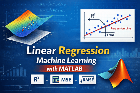
Linear Regression is one of the most important machine learning algorithms for predicting continuous values. In MATLAB, the main function for fitting linear regression models is fitlm, which returns a LinearModel object you can inspect, evaluate, and use for prediction. MATLAB also provides related tools such as predict, stepwiselm, regress, and the Regression Learner app for GUI-based workflows.
This tutorial explains the theory of linear regression, how it works, when to use it, and how to implement it in MATLAB with practical examples.
1. What is Linear Regression?
Linear Regression is a supervised learning method used to model the relationship between a response variable and one or more predictor variables. The goal is to predict a continuous output such as price, salary, temperature, or sales. MathWorks defines a linear regression model as one that describes the relationship between a dependent variable y and one or more independent variables X.
In simple terms:
- Simple Linear Regression uses one predictor.
- Multiple Linear Regression uses two or more predictors.
A general linear regression equation looks like this:
$y = b_0 + b_1x_1 + b_2x_2 + \dots + b_nx_n$
where:
yis the predicted output,b0is the intercept,b1, b2, ...are coefficients,x1, x2, ...are predictor values
2. Why use Linear Regression?
Linear Regression is popular because it is:
- simple to understand,
- easy to implement,
- fast to train,
- interpretable,
- useful as a baseline model.
It is especially useful when the target variable is numeric and when the relationship between predictors and the response is approximately linear.
3. Main concepts behind Linear Regression
3.1 Response variable
This is the output you want to predict, such as house price.
3.2 Predictor variables
These are the inputs used to explain or predict the response.
3.3 Intercept
The intercept is the predicted value of y when all predictors are zero.
3.4 Coefficients
Each coefficient tells you how much the response changes when the corresponding predictor changes by one unit, while the other predictors stay fixed.
3.5 Residuals
Residuals are the differences between real values and predicted values:
Residual=yactual−ypredicted\text{Residual} = y_{\text{actual}} - y_{\text{predicted}}Residual=yactual−ypredicted
Residual analysis is an important part of assessing model quality, and MathWorks recommends checking residual plots and goodness-of-fit measures such as R^2 and adjusted R^2.
4. MATLAB functions you need to know
The main MATLAB functions and tools for linear regression are:
fitlm→ fit linear regression modelspredict→ predict outputs for new datastepwiselm→ build models with stepwise variable selectionregress→ classical multiple linear regression functionRegression Learnerapp → visual interface for regression modelingLinearModelobject → inspect coefficients, fitted values, residuals, and model statistics
Part I — Simple Linear Regression in MATLAB
5. First example: one predictor and one response
Let us begin with a simple dataset where one variable predicts another.
clc;
clear;
close all;

% Example data
X = [1; 2; 3; 4; 5; 6];
Y = [2; 4; 5; 4; 5; 7];

% Fit linear regression model
mdl = fitlm(X, Y);

% Display model
disp(mdl);
Explanation
Here:
Xcontains one predictor,Ycontains the output values,fitlm(X,Y)fits a linear regression model.
According to MathWorks, fitlm(X,y) returns a linear regression model fit to predictor matrix X and response y.
6. Plotting the regression line
clc;
clear;
close all;

X = [1; 2; 3; 4; 5; 6];
Y = [2; 4; 5; 4; 5; 7];

mdl = fitlm(X, Y);

% Scatter plot of data
plot(X, Y, 'o');
hold on;

% Predicted values
YPred = predict(mdl, X);

% Regression line
plot(X, YPred, '-');
xlabel('X');
ylabel('Y');
title('Simple Linear Regression');
legend('Data', 'Regression Line');
grid on;
This is often the first useful visualization: points show the real data and the line shows the fitted linear trend.
7. Understanding the model output
When you display mdl, MATLAB gives information such as:
- the fitted formula,
- estimated coefficients,
- standard errors,
- t-statistics,
- p-values,
R-squared.
MathWorks provides dedicated documentation for interpreting linear regression outputs and understanding the coefficient table and goodness-of-fit statistics.
Example:
disp(mdl.Coefficients);This displays the coefficient table.
8. Predicting new values
Once the model is trained, you can predict outputs for new observations using predict.
clc;
clear;
close all;

X = [1; 2; 3; 4; 5; 6];
Y = [2; 4; 5; 4; 5; 7];

mdl = fitlm(X, Y);

% New predictor values
Xnew = [7; 8; 9];

% Predict
YPredNew = predict(mdl, Xnew);

disp('Predicted values:');
disp(YPredNew);
MathWorks documents predict(mdl,Xnew) as the standard way to return predicted responses from a linear regression model.
Part II — Multiple Linear Regression in MATLAB
9. What is multiple linear regression?
Multiple linear regression uses more than one predictor.
Example idea:
x1= size of a housex2= number of roomsx3= age of the housey= price
The model becomes:
$y = b_0 + b_1x_1 + b_2x_2 + b_3x_3$
10. Multiple regression example in MATLAB
clc;
clear;
close all;

% Predictor matrix: columns are features
X = [1 5;
     2 4;
     3 6;
     4 8;
     5 7;
     6 9];

% Response
Y = [10; 12; 13; 16; 17; 20];

% Fit multiple linear regression
mdl = fitlm(X, Y);

disp(mdl);
Here:
- column 1 and column 2 are predictors,
fitlmautomatically handles multiple predictors whenXhas multiple columns.
11. Multiple regression with a table
MATLAB works very well with tables, which often makes code more readable.
clc;
clear;
close all;

Size = [50; 60; 70; 80; 90; 100];
Rooms = [2; 3; 3; 4; 4; 5];
Price = [100; 120; 140; 160; 180; 210];

tbl = table(Size, Rooms, Price);

mdl = fitlm(tbl, 'Price ~ Size + Rooms');

disp(mdl);
MathWorks documents fitlm(tbl) and formula-based workflows such as fitlm(tbl,modelspec) for table inputs. It also notes that when you pass a table without specifying otherwise, the last variable is treated as the response.
12. Making predictions from multiple predictors
clc;
clear;
close all;

Size = [50; 60; 70; 80; 90; 100];
Rooms = [2; 3; 3; 4; 4; 5];
Price = [100; 120; 140; 160; 180; 210];

tbl = table(Size, Rooms, Price);

mdl = fitlm(tbl, 'Price ~ Size + Rooms');

newData = table([75; 95], [3; 5], 'VariableNames', {'Size','Rooms'});

YPred = predict(mdl, newData);

disp('Predicted prices:');
disp(YPred);
Part III — Evaluating Linear Regression Models
13. R-squared
One of the most common measures of regression quality is R-squared. It measures how much of the variability in the response is explained by the model.
In MATLAB:
mdl.RsquaredMathWorks highlights R^2 and adjusted R^2 as core goodness-of-fit measures in linear regression analysis.
Example:
clc;
clear;
close all;

X = [1; 2; 3; 4; 5; 6];
Y = [2; 4; 5; 4; 5; 7];

mdl = fitlm(X, Y);

disp('R-squared:');
disp(mdl.Rsquared.Ordinary);

disp('Adjusted R-squared:');
disp(mdl.Rsquared.Adjusted);
14. MAE, MSE, and RMSE
These are very common regression metrics:
- MAE = Mean Absolute Error
- MSE = Mean Squared Error
- RMSE = Root Mean Squared Error
clc;
clear;
close all;

X = [1; 2; 3; 4; 5; 6];
Y = [2; 4; 5; 4; 5; 7];

mdl = fitlm(X, Y);
YPred = predict(mdl, X);

MAE = mean(abs(Y - YPred));
MSE = mean((Y - YPred).^2);
RMSE = sqrt(MSE);

fprintf('MAE  = %.4f\n', MAE);
fprintf('MSE  = %.4f\n', MSE);
fprintf('RMSE = %.4f\n', RMSE);
These metrics are especially useful when comparing several regression models.
15. Residual analysis
Residual plots help you understand whether the model assumptions are reasonable.
clc;
clear;
close all;

X = [1; 2; 3; 4; 5; 6];
Y = [2; 4; 5; 4; 5; 7];

mdl = fitlm(X, Y);

figure;
plotResiduals(mdl, 'fitted');
title('Residuals vs Fitted Values');

figure;
plotResiduals(mdl, 'probability');
title('Normal Probability Plot of Residuals');
MathWorks specifically recommends examining residuals and looking for patterns when assessing the quality of a linear regression fit.
Part IV — Train/Test Split Workflow
16. Why train/test split matters
A model may fit the training data well but still perform poorly on new unseen data. That is why a train/test split is important in machine learning.
17. Example with train/test split
clc;
clear;
close all;

% Example dataset
X = [1; 2; 3; 4; 5; 6; 7; 8; 9; 10];
Y = [1.2; 2.1; 2.9; 4.1; 5.2; 5.9; 7.1; 8.2; 8.8; 10.1];

% Split index
rng(1);
idx = randperm(length(X));

trainIdx = idx(1:7);
testIdx  = idx(8:end);

XTrain = X(trainIdx);
YTrain = Y(trainIdx);

XTest = X(testIdx);
YTest = Y(testIdx);

% Train model
mdl = fitlm(XTrain, YTrain);

% Predict on test set
YPred = predict(mdl, XTest);

% Test RMSE
RMSE = sqrt(mean((YTest - YPred).^2));
fprintf('Test RMSE = %.4f\n', RMSE);

% Compare real and predicted
disp(table(XTest, YTest, YPred));
This simple workflow is a good starting point for practical machine learning projects.
Part V — A Real MATLAB Dataset Example
18. Example with the carsmall dataset
MATLAB includes several built-in datasets. One well-known example for regression is carsmall.
clc;
clear;
close all;

load carsmall

% Create table
tbl = table(Horsepower, Weight, MPG);

% Remove missing values
tbl = rmmissing(tbl);

% Fit model: predict MPG using Horsepower and Weight
mdl = fitlm(tbl, 'MPG ~ Horsepower + Weight');

disp(mdl);

% Predicted MPG
YPred = predict(mdl, tbl(:, {'Horsepower','Weight'}));

% Plot actual vs predicted
figure;
plot(tbl.MPG, YPred, 'o');
xlabel('Actual MPG');
ylabel('Predicted MPG');
title('Actual vs Predicted MPG');
grid on;
This is a more realistic example of multiple linear regression.
19. Example with interaction terms
Sometimes the effect of one predictor depends on another. In that case, you can include interaction terms.
clc;
clear;
close all;

load carsmall

tbl = table(Horsepower, Weight, MPG);
tbl = rmmissing(tbl);

mdl = fitlm(tbl, 'MPG ~ Horsepower * Weight');

disp(mdl);
Formula syntax in fitlm supports model specifications and interactions, which is one of the reasons the LinearModel workflow is flexible.
Part VI — Stepwise Linear Regression
20. Why stepwise regression?
When you have many predictors, not all of them may be useful. Stepwise regression is a variable selection method that adds or removes predictors iteratively.
MathWorks describes stepwise regression as a dimensionality-reduction method where less important variables are successively removed in an automatic iterative process, and it can be done with stepwiselm, stepwisefit, or the Regression Learner app.
21. Stepwise regression example
clc;
clear;
close all;

load carsmall

tbl = table(Horsepower, Weight, Acceleration, MPG);
tbl = rmmissing(tbl);

mdl = stepwiselm(tbl, 'MPG ~ 1', 'Upper', 'linear');

disp(mdl);
This allows MATLAB to test which predictors improve the model.
Part VII — Using regress
22. Classical regression with regress
MATLAB also has the function regress, but MathWorks notes that fitlm is usually preferable when you want a richer model object and more analysis tools.
Example:
clc;
clear;
close all;

X = [1; 2; 3; 4; 5; 6];
Y = [2; 4; 5; 4; 5; 7];

% Add intercept column
Xreg = [ones(size(X)) X];

[b, bint, r, rint, stats] = regress(Y, Xreg);

disp('Coefficients:');
disp(b);

disp('Stats [R2 F p error variance]:');
disp(stats);
This is more classical and lower-level than fitlm.
Part VIII — Regression Learner App
23. GUI-based regression in MATLAB
MATLAB provides the Regression Learner app, which lets you import data, choose validation schemes, train models, optimize hyperparameters, compare results, and inspect predictor contributions.
To open it:
regressionLearnerTypical steps:
- open the app,
- import your dataset,
- choose the response variable,
- select linear regression models,
- train and compare them,
- export the best model or generated code.
This is very useful for beginners.
Part IX — End-to-End Mini Project
24. Project: Predict house prices
Let us build a small end-to-end linear regression project.
clc;
clear;
close all;

% Example house dataset
Size = [50; 60; 70; 80; 90; 100; 110; 120];
Rooms = [2; 3; 3; 4; 4; 5; 5; 6];
Age = [20; 18; 15; 12; 10; 8; 5; 3];
Price = [100; 120; 135; 150; 170; 190; 210; 230];

tbl = table(Size, Rooms, Age, Price);

% Train/test split
rng(2);
idx = randperm(height(tbl));

trainIdx = idx(1:6);
testIdx  = idx(7:8);

trainTbl = tbl(trainIdx, :);
testTbl  = tbl(testIdx, :);

% Train model
mdl = fitlm(trainTbl, 'Price ~ Size + Rooms + Age');

disp(mdl);

% Predict
YPred = predict(mdl, testTbl(:, {'Size','Rooms','Age'}));

% Evaluate
YTest = testTbl.Price;
RMSE = sqrt(mean((YTest - YPred).^2));
MAE = mean(abs(YTest - YPred));

fprintf('Test RMSE = %.4f\n', RMSE);
fprintf('Test MAE  = %.4f\n', MAE);

% Show results
disp(table(YTest, YPred));

% Predict a new house
newHouse = table(95, 4, 7, 'VariableNames', {'Size','Rooms','Age'});
newPrice = predict(mdl, newHouse);

fprintf('Predicted price for new house = %.2f\n', newPrice);
What this project teaches
This project covers:
- building a dataset,
- splitting train/test,
- fitting a linear regression model,
- making predictions,
- evaluating the model,
- predicting new unseen observations.
That is a strong beginner workflow.
Part X — Common mistakes in Linear Regression
25. Using linear regression for classification
Linear Regression is for continuous outputs, not class labels.
26. Ignoring residuals
A high R^2 is not enough. Residual plots can reveal model problems.
27. Using too many predictors without checking relevance
This can lead to unnecessary complexity. Stepwise methods or thoughtful feature selection can help.
28. Predicting outside the meaningful data range
Extrapolation can produce unreliable predictions.
29. Assuming correlation always means causation
A useful predictive relationship does not automatically imply a causal relationship.
Part XI — When should you use Linear Regression?
Linear Regression is a good choice when:
- the target is numeric,
- you want a simple and interpretable model,
- the relationship is approximately linear,
- you need a strong baseline model.
You may choose another model when:
- the relationship is highly nonlinear,
- there are complex interactions you cannot model well linearly,
- errors are structured in ways that violate simple regression assumptions.
Part XII — Summary
Linear Regression is one of the best starting points in machine learning. In MATLAB, the standard workflow uses fitlm to fit the model, predict to generate outputs, residual plots and R^2 to evaluate quality, and tools such as stepwiselm or Regression Learner for model improvement and exploration. MathWorks also positions fitlm as a central least-squares workflow for linear regression analysis and documents it as the typical training path for linear regression models.
A practical workflow is:
- prepare the dataset,
- fit the model with
fitlm, - inspect coefficients and significance,
- evaluate residuals and goodness of fit,
- test on unseen data,
- use the model for prediction.
Part XIII — MATLAB cheat sheet
Simple linear regression
mdl = fitlm(X, Y);Multiple linear regression
mdl = fitlm(X, Y);Table-based regression
mdl = fitlm(tbl, 'Y ~ X1 + X2');Prediction
YPred = predict(mdl, Xnew);Stepwise regression
mdl = stepwiselm(tbl, 'Y ~ 1', 'Upper', 'linear');Classical regression
[b, bint, r, rint, stats] = regress(Y, Xreg);Open Regression Learner
regressionLearnerPractice exercises
Exercise 1
Fit a simple linear regression model using one predictor and plot the regression line
Exercise 2
Use two predictors in a multiple linear regression model and display the coefficients
Exercise 3
Split a dataset into training and test sets, train a model, and compute RMSE
Exercise 4
Use the carsmall dataset to predict MPG from Horsepower and Weight
Exercise 5
Use stepwiselm to select useful predictors for a regression problem
Short recap
Exercise 1
Simple linear regression with one predictor and a regression line plot.
Exercise 2
Multiple linear regression with two predictors and coefficient display.
Exercise 3
Train/test split and RMSE calculation.
Exercise 4
Real regression example using the carsmall dataset.
Exercise 5
Automatic predictor selection using stepwiselm.










💬 Comments
No comments yet. Be the first to comment!
Login to comment.