
0) Introduction
XGBoost is a gradient-boosting library for supervised learning that is widely used for classification and regression. In Python, the most common estimators are XGBClassifier and XGBRegressor. The official docs describe XGBoost as an optimized gradient boosting library that provides parallel tree boosting for fast and accurate modeling.
1) What XGBoost does
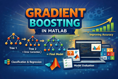
XGBoost builds an ensemble of trees sequentially. It starts with a simple model, measures the current errors, then adds a new tree that tries to correct those errors. The final prediction is the sum of the contributions from many trees. This is the same boosting idea you saw in Gradient Boosting, but XGBoost adds strong engineering and regularization features that make it especially effective in practice.
For classification, the model predicts a class or class probabilities. For regression, it predicts a numeric value. In the Python API, these tasks are handled by xgboost.XGBClassifier and xgboost.XGBRegressor.
2) Why XGBoost is popular
XGBoost is popular because it often performs very well on tabular data, handles nonlinear relationships, supports regularization, and offers CPU and GPU training options. The official docs also note support for GPU training through the device parameter.
In practice, XGBoost is often chosen when:
- you want strong predictive performance
- your features interact in complex ways
- you are working with structured data
- you are willing to tune the model carefully
Those strengths come from the boosting framework plus the additional controls exposed in XGBoost’s parameter system.
3) XGBoost vs classical Gradient Boosting
Both are boosting methods, but XGBoost is more specialized and more optimized. Classical gradient boosting in scikit-learn builds trees stage by stage using gradients of the loss, while XGBoost adds its own parameter system, regularization controls, optimized training implementation, and broader system support.
A useful practical distinction is this:
- Gradient Boosting in scikit-learn is a great way to learn the idea
- XGBoost is a more advanced production-oriented implementation of boosted trees
That is an inference from the official descriptions of each library’s boosting framework and capabilities.
4) Core intuition
Think of XGBoost as building many small corrective trees. Each new tree tries to improve what the current ensemble is still getting wrong. Over time, the model becomes stronger by adding many small improvements instead of relying on one large tree.
This means the important ideas are:
- boosting: add trees one after another
- weak learners: usually shallow trees
- learning rate: control how much each new tree changes the model
- regularization: reduce overfitting
XGBoost’s official parameters page separates configuration into general, booster, and learning-task parameters, which reflects this design.
5) Important XGBoost parameters
Some of the most important parameters in practice are:
n_estimators: number of treeslearning_rate: shrinkage factormax_depth: maximum tree depthsubsample: row samplingcolsample_bytree: feature sampling per treereg_alpha: L1 regularizationreg_lambda: L2 regularizationobjective: learning taskeval_metric: evaluation metricdevice: CPU or GPU choice in modern XGBoost
These parameters matter because they control model complexity, how aggressively the model learns, and how much randomness and regularization are applied.
6) Learning rate and number of trees
The interaction between learning_rate and n_estimators is one of the most important tuning choices.
- smaller
learning_rateusually means safer, slower learning - smaller
learning_rateoften requires more trees - larger
learning_ratecan converge faster but may overfit more easily
This is a standard consequence of boosted additive models, and XGBoost exposes both controls directly in its parameter system.
7) Tree depth and overfitting
max_depth controls how complex each tree can become.
- small depth → simpler learners
- large depth → more expressive learners
- very large depth → higher overfitting risk
Because XGBoost adds many trees, allowing each one to become too large can make the full model overly complex. That follows directly from the booster parameter controls in the official docs.
8) Subsampling and column sampling
XGBoost can randomly sample both rows and features.
subsamplecontrols the fraction of training rows usedcolsample_bytreecontrols the fraction of features used per tree
These are useful regularization tools because they reduce correlation and can help generalization. They are official booster parameters in XGBoost.
9) Regularization in XGBoost
One reason XGBoost is powerful is that it includes explicit regularization terms.
reg_alphaadds L1 regularizationreg_lambdaadds L2 regularization
These are documented booster parameters in XGBoost and are part of what distinguishes it from simpler boosting implementations.
10) Do you need feature scaling?
For tree-based XGBoost models, feature scaling is usually not necessary, because tree splits are threshold-based rather than distance-based. This is an inference from the fact that XGBClassifier and XGBRegressor are boosted tree estimators, like other tree-based methods.
So unlike KNN or SVM, you usually do not start with StandardScaler for tree-based XGBoost.
Part I — Installation
11) Install the required libraries
pip install xgboost scikit-learn numpy pandas matplotlibThe XGBoost Python docs describe the Python package as having multiple interfaces, including the scikit-learn interface, which is what we will use here.
Part II — First Classification Example
12) Train an XGBClassifier
We will use the Breast Cancer dataset from scikit-learn.
import numpy as np
import pandas as pd

from sklearn.datasets import load_breast_cancer
from sklearn.model_selection import train_test_split
from sklearn.metrics import accuracy_score, classification_report, confusion_matrix
from xgboost import XGBClassifier

# Load dataset
data = load_breast_cancer()
X = data.data
y = data.target

# Split
X_train, X_test, y_train, y_test = train_test_split(
    X, y, test_size=0.2, random_state=42, stratify=y
)

# Build model
model = XGBClassifier(
    n_estimators=200,
    learning_rate=0.05,
    max_depth=4,
    subsample=0.8,
    colsample_bytree=0.8,
    objective="binary:logistic",
    eval_metric="logloss",
    random_state=42
)

# Train
model.fit(X_train, y_train)

# Predict
y_pred = model.predict(X_test)

# Evaluate
print("Accuracy:", accuracy_score(y_test, y_pred))
print("\nConfusion Matrix:\n", confusion_matrix(y_test, y_pred))
print("\nClassification Report:\n", classification_report(y_test, y_pred))
train_test_split is the standard scikit-learn utility for splitting data into train and test subsets, classification_report summarizes precision, recall, and F1-style metrics, and confusion_matrix evaluates classification results in matrix form.
13) What this code does
This workflow:
- loads the data
- creates training and test sets
- fits an XGBoost classifier
- predicts test labels
- evaluates the results with accuracy, confusion matrix, and classification report
The classification metrics used here are standard scikit-learn evaluation tools, and XGBClassifier is part of the official XGBoost Python API.
14) Predicting probabilities
Like many classifiers, XGBoost can return probabilities.
proba = model.predict_proba(X_test[:5])
print(proba)
This is useful when you care not only about the predicted class, but also about how confident the model is. XGBClassifier exposes standard classifier methods like fit, predict, and probability-style prediction in the Python API.
Part III — Important Classification Parameters
15) The most useful ones to tune
For XGBClassifier, the most common parameters to tune are:
n_estimatorslearning_ratemax_depthsubsamplecolsample_bytreereg_alphareg_lambda- sometimes
min_child_weightandgammafor additional tree regularization
These parameters control how many trees the model uses, how large the trees are, how aggressively it learns, and how strongly it regularizes.
16) A safer starting configuration
A practical baseline often looks like this:
model = XGBClassifier(
    n_estimators=300,
    learning_rate=0.05,
    max_depth=4,
    subsample=0.8,
    colsample_bytree=0.8,
    reg_alpha=0.0,
    reg_lambda=1.0,
    objective="binary:logistic",
    eval_metric="logloss",
    random_state=42
)
This is not a universal best configuration, but it is a sensible starting point based on the official XGBoost booster parameters and common boosting practice.
Part IV — Feature Importance
17) Built-in feature importance
XGBoost models can report feature importances.
import pandas as pd

importance = pd.Series(model.feature_importances_, index=data.feature_names)
print(importance.sort_values(ascending=False))
This can help you see which variables the model used most strongly. The scikit-learn style XGBoost estimators expose feature_importances_ in the Python API.
18) Plot feature importance
import matplotlib.pyplot as plt

importance = importance.sort_values(ascending=True)

plt.figure(figsize=(8, 6))
importance.plot(kind="barh")
plt.title("XGBoost Feature Importance")
plt.xlabel("Importance")
plt.ylabel("Feature")
plt.show()
This is useful for interpretation, though model-based importance should still be treated carefully as a model summary rather than proof of causality. That caution is an inference based on how tree-based importance values are constructed.
Part V — Hyperparameter Tuning
19) Tune with GridSearchCV
Scikit-learn’s GridSearchCV performs an exhaustive search over parameter combinations.
from sklearn.model_selection import GridSearchCV
from xgboost import XGBClassifier

param_grid = {
    "n_estimators": [100, 200, 300],
    "learning_rate": [0.01, 0.05, 0.1],
    "max_depth": [3, 4, 5],
    "subsample": [0.8, 1.0],
    "colsample_bytree": [0.8, 1.0]
}

grid = GridSearchCV(
    estimator=XGBClassifier(
        objective="binary:logistic",
        eval_metric="logloss",
        random_state=42
    ),
    param_grid=param_grid,
    cv=5,
    scoring="accuracy",
    n_jobs=-1
)

grid.fit(X_train, y_train)

print("Best Parameters:", grid.best_params_)
print("Best CV Score:", grid.best_score_)

best_model = grid.best_estimator_
y_pred = best_model.predict(X_test)
print("Test Accuracy:", accuracy_score(y_test, y_pred))
This is one of the best practical ways to choose a strong XGBoost configuration.
20) What to tune first
A good order of priority is often:
learning_raten_estimatorsmax_depthsubsamplecolsample_bytree- regularization terms like
reg_alphaandreg_lambda
That ordering is a practical inference based on the official XGBoost parameter groups and the way boosting models typically behave.
Part VI — XGBoost Regression
21) Train an XGBRegressor
Now let us use XGBoost for regression.
import numpy as np
import matplotlib.pyplot as plt

from sklearn.model_selection import train_test_split
from sklearn.metrics import mean_squared_error, r2_score
from xgboost import XGBRegressor

# Synthetic data
rng = np.random.RandomState(42)
X = np.sort(5 * rng.rand(200, 1), axis=0)
y = np.sin(X).ravel()

# Add noise
y[::5] += 0.5 - rng.rand(40)

X_train, X_test, y_train, y_test = train_test_split(
    X, y, test_size=0.2, random_state=42
)

model = XGBRegressor(
    n_estimators=300,
    learning_rate=0.05,
    max_depth=4,
    subsample=0.8,
    colsample_bytree=0.8,
    objective="reg:squarederror",
    random_state=42
)

model.fit(X_train, y_train)
y_pred = model.predict(X_test)

print("MSE:", mean_squared_error(y_test, y_pred))
print("R²:", r2_score(y_test, y_pred))
XGBRegressor is the regression counterpart in the XGBoost Python API, while mean_squared_error and r2_score are standard scikit-learn regression metrics.
22) Plot regression predictions
X_plot = np.linspace(X.min(), X.max(), 500).reshape(-1, 1)
y_plot = model.predict(X_plot)

plt.figure(figsize=(8, 6))
plt.scatter(X, y, label="Data")
plt.plot(X_plot, y_plot, linewidth=2, label="XGBoost prediction")
plt.xlabel("X")
plt.ylabel("y")
plt.title("XGBoost Regression")
plt.legend()
plt.show()
This kind of example is useful for seeing how boosting can model a nonlinear curve from many tree-based corrections. That is a direct consequence of XGBoost’s boosted-tree formulation.
Part VII — Full Real Workflow
23) End-to-end classification workflow
Step 1: Load data
import pandas as pd

df = pd.read_csv("your_data.csv")
Step 2: Separate features and target
X = df.drop("target", axis=1)
y = df["target"]
Step 3: Split data
from sklearn.model_selection import train_test_split

X_train, X_test, y_train, y_test = train_test_split(
    X, y, test_size=0.2, random_state=42, stratify=y
)
Step 4: Build model
from xgboost import XGBClassifier

model = XGBClassifier(
    objective="binary:logistic",
    eval_metric="logloss",
    random_state=42
)
Step 5: Tune parameters
from sklearn.model_selection import GridSearchCV

param_grid = {
    "n_estimators": [100, 200],
    "learning_rate": [0.05, 0.1],
    "max_depth": [3, 4, 5],
    "subsample": [0.8, 1.0],
    "colsample_bytree": [0.8, 1.0]
}

grid = GridSearchCV(
    model,
    param_grid=param_grid,
    cv=5,
    scoring="accuracy",
    n_jobs=-1
)

grid.fit(X_train, y_train)
Step 6: Evaluate
from sklearn.metrics import classification_report, confusion_matrix, accuracy_score

best_model = grid.best_estimator_
y_pred = best_model.predict(X_test)

print("Best Params:", grid.best_params_)
print("Accuracy:", accuracy_score(y_test, y_pred))
print(confusion_matrix(y_test, y_pred))
print(classification_report(y_test, y_pred))
This follows the standard scikit-learn estimator workflow for train/test splitting, cross-validated search, and classification evaluation.
Part VIII — Categorical Data
24) XGBoost and categorical features
The official XGBoost docs note that one easy way to pass categorical data is through a dataframe using the scikit-learn interface, with columns explicitly marked as category dtype.
Example idea:
import pandas as pd
from xgboost import XGBClassifier

X["cat_feature"] = X["cat_feature"].astype("category")

model = XGBClassifier(
    tree_method="hist",
    enable_categorical=True,
    objective="binary:logistic",
    eval_metric="logloss"
)
This is a useful modern feature in XGBoost when your data includes categorical columns.
Part IX — GPU Support
25) Using GPU
The XGBoost docs state that to enable GPU support, you can set the device parameter to cuda or gpu in the Python API.
Example:
model = XGBClassifier(
    n_estimators=300,
    learning_rate=0.05,
    max_depth=4,
    objective="binary:logistic",
    eval_metric="logloss",
    device="cuda",
    random_state=42
)
This can speed up training substantially on supported hardware.
Part X — How to Read Results
26) Classification metrics
For classification, the most common metrics are:
- accuracy
- precision
- recall
- F1-score
- confusion matrix
Scikit-learn provides classification_report and confusion_matrix for these tasks.
from sklearn.metrics import confusion_matrix, classification_report

print(confusion_matrix(y_test, y_pred))
print(classification_report(y_test, y_pred))
27) Regression metrics
For regression, common metrics include:
- MAE
- MSE
- RMSE
- R²
These are standard scikit-learn regression evaluation tools.
from sklearn.metrics import mean_absolute_error, mean_squared_error, r2_score
import numpy as np

mae = mean_absolute_error(y_test, y_pred)
mse = mean_squared_error(y_test, y_pred)
rmse = np.sqrt(mse)
r2 = r2_score(y_test, y_pred)

print("MAE:", mae)
print("MSE:", mse)
print("RMSE:", rmse)
print("R²:", r2)
Part XI — Strengths and Weaknesses
28) Strengths of XGBoost
XGBoost is strong because it offers:
- boosted trees with high predictive power
- strong regularization controls
- CPU and GPU support
- a scikit-learn-compatible interface
- support for categorical workflows in modern usage
These features are part of why it remains a standard choice for many tabular machine learning tasks.
29) Weaknesses of XGBoost
Its main limitations are:
- it usually needs tuning
- it is less interpretable than a single tree
- training can become expensive with large search spaces
- careless parameter choices can overfit
These are practical consequences of using a flexible boosted ensemble with many interacting parameters.
Part XII — Common Mistakes
30) Using too high a learning rate
Bad:
model = XGBClassifier(
    n_estimators=500,
    learning_rate=0.5,
    objective="binary:logistic",
    eval_metric="logloss"
)
Better:
model = XGBClassifier(
    n_estimators=300,
    learning_rate=0.05,
    max_depth=4,
    subsample=0.8,
    colsample_bytree=0.8,
    objective="binary:logistic",
    eval_metric="logloss"
)
That advice follows from the role of shrinkage and stage count in boosted models.
31) Ignoring regularization
Many beginners tune only n_estimators and max_depth, but XGBoost also provides subsample, colsample_bytree, reg_alpha, and reg_lambda, which are important for controlling overfitting.
32) Searching too many combinations at once
GridSearchCV is exhaustive, so the search can become slow if the grid is too large. The scikit-learn docs explicitly describe it as trying all parameter combinations, and also note alternatives like RandomizedSearchCV.
So start with a modest grid, then refine around promising values.
Part XIII — Practical Advice
33) When should you use XGBoost?
Use XGBoost when:
- you want strong performance on structured data
- you are comfortable tuning hyperparameters
- nonlinear relationships matter
- you want a robust boosting method with mature tooling
34) When should you avoid it?
Be cautious when:
- interpretability is your top priority
- you need the simplest possible baseline
- you do not have time to tune
- a lighter model would already solve the problem
Those are practical tradeoffs of a powerful but flexible ensemble method.
35) Good default starting points
For binary classification:
XGBClassifier(
    n_estimators=300,
    learning_rate=0.05,
    max_depth=4,
    subsample=0.8,
    colsample_bytree=0.8,
    objective="binary:logistic",
    eval_metric="logloss",
    random_state=42
)
For regression:
XGBRegressor(
    n_estimators=300,
    learning_rate=0.05,
    max_depth=4,
    subsample=0.8,
    colsample_bytree=0.8,
    objective="reg:squarederror",
    random_state=42
)
These are sensible baselines based on the official XGBoost parameter families, not guaranteed best settings.
Part XIV — Mini Project Example
36) Predicting iris species with XGBoost
from sklearn.datasets import load_iris
from sklearn.model_selection import train_test_split, GridSearchCV
from sklearn.metrics import classification_report, confusion_matrix, accuracy_score
from xgboost import XGBClassifier

# Load
data = load_iris()
X, y = data.data, data.target

# Split
X_train, X_test, y_train, y_test = train_test_split(
    X, y, test_size=0.2, stratify=y, random_state=42
)

# Model
model = XGBClassifier(
    objective="multi:softprob",
    num_class=3,
    eval_metric="mlogloss",
    random_state=42
)

# Search space
param_grid = {
    "n_estimators": [100, 200, 300],
    "learning_rate": [0.01, 0.05, 0.1],
    "max_depth": [3, 4, 5],
    "subsample": [0.8, 1.0],
    "colsample_bytree": [0.8, 1.0]
}

# Grid search
grid = GridSearchCV(
    model,
    param_grid=param_grid,
    cv=5,
    scoring="accuracy",
    n_jobs=-1
)

grid.fit(X_train, y_train)

# Evaluate
best_model = grid.best_estimator_
y_pred = best_model.predict(X_test)

print("Best Parameters:", grid.best_params_)
print("Accuracy:", accuracy_score(y_test, y_pred))
print("\nConfusion Matrix:\n", confusion_matrix(y_test, y_pred))
print("\nClassification Report:\n", classification_report(y_test, y_pred))
This example combines XGBoost’s scikit-learn interface with scikit-learn’s split, search, and evaluation tools in a standard workflow.
Part XV — Summary
37) What you should remember
XGBoost is a powerful boosted-tree method for classification and regression. It builds trees sequentially, each one trying to improve the current model, and it provides practical controls for shrinkage, sampling, regularization, and hardware acceleration.
The most important practical rules are:
- feature scaling is usually not needed for tree-based XGBoost
- tune
learning_rateandn_estimatorstogether - control complexity with
max_depth - use
subsampleandcolsample_bytree - do not ignore
reg_alphaandreg_lambda - use cross-validation for tuning
38) Final ready-to-use template
from sklearn.model_selection import train_test_split, GridSearchCV
from sklearn.metrics import classification_report
from xgboost import XGBClassifier

# X, y = your data

X_train, X_test, y_train, y_test = train_test_split(
    X, y, test_size=0.2, random_state=42
)

model = XGBClassifier(
    objective="binary:logistic",
    eval_metric="logloss",
    random_state=42
)

param_grid = {
    "n_estimators": [100, 200],
    "learning_rate": [0.05, 0.1],
    "max_depth": [3, 4, 5],
    "subsample": [0.8, 1.0],
    "colsample_bytree": [0.8, 1.0]
}

grid = GridSearchCV(
    model,
    param_grid=param_grid,
    cv=5,
    scoring="accuracy",
    n_jobs=-1
)

grid.fit(X_train, y_train)

print("Best params:", grid.best_params_)
print("Test score:", grid.best_estimator_.score(X_test, y_test))

y_pred = grid.best_estimator_.predict(X_test)
print(classification_report(y_test, y_pred))
39) Practice exercises
Exercise 1
Train an XGBClassifier on the Iris dataset and report accuracy.
Exercise 2
Train XGBoost on the Breast Cancer dataset and display feature importances.
Exercise 3
Tune learning_rate, n_estimators, and max_depth using GridSearchCV.
Exercise 4
Compare a RandomForestClassifier with an XGBClassifier.
Exercise 5
Train an XGBRegressor on a nonlinear synthetic regression dataset.
Final summary
What each exercise teaches
- Exercise 1: basic XGBoost classification
- Exercise 2: feature importance analysis
- Exercise 3: hyperparameter tuning with cross-validation
- Exercise 4: comparison between Random Forest and XGBoost
- Exercise 5: nonlinear regression with XGBoost









💬 Comments
No comments yet. Be the first to comment!
Login to comment.