0) Introduction
K-Nearest Neighbors, or KNN, is a supervised machine learning method used for both classification and regression. In scikit-learn, the main classes are KNeighborsClassifier and KNeighborsRegressor. The nearest-neighbors family predicts from nearby examples in the training set rather than learning a parametric equation, which is why it is often described as an instance-based or lazy learning method.
1) What KNN does
KNN makes predictions by looking at the closest training samples to a new point. For classification, it uses the neighbors’ class labels to vote on the prediction. For regression, it predicts from the target values of the nearby samples. Scikit-learn’s user guide describes KNeighborsClassifier as classification based on the k nearest neighbors of each query point, and KNeighborsRegressor as regression based on the k nearest neighbors of each query point.
Imagine you want to classify a fruit using only:
- weight
- color score
If a new fruit is surrounded mostly by apples in feature space, KNN will likely classify it as an apple. If its closest neighbors are mostly oranges, it will likely predict orange.
That is the core idea:
- store the training data
- measure distance from the new point to the training points
- choose the nearest
kpoints - aggregate their labels or values
2) Why KNN is useful
KNN is a popular first algorithm because it is simple, intuitive, and often effective on small to medium datasets. It is also flexible because the same idea works for both classification and regression. In scikit-learn, you can choose how many neighbors to use, how to weight them, and which distance metric to apply.
KNN is especially useful when:
- the decision boundary is nonlinear
- the dataset is not huge
- you want an easy baseline
- you want a model that is easy to explain
3) The meaning of k
The parameter k is the number of nearest neighbors considered when making a prediction. In scikit-learn, this is the n_neighbors parameter, whose default is 5 for both KNeighborsClassifier and KNeighborsRegressor.
Small k
If k is very small, such as 1:
- the model becomes very sensitive to noise
- it can fit the training data too closely
- it may overfit
Large k
If k is large:
- the model becomes smoother
- it is less sensitive to noise
- it may underfit
So choosing k is a balance between:
- flexibility
- stability
4) How KNN classification works
Suppose you have two classes:
- class 0
- class 1
For a new point:
- compute the distance to every training point
- select the closest
k - count the class labels
- predict the majority class
Scikit-learn describes KNeighborsClassifier as implementing the vote of the nearest neighbors, and it exposes methods such as kneighbors to inspect the nearest samples and their distances.
Example
If k = 5 and the 5 nearest neighbors are:
- 3 from class A
- 2 from class B
Then the prediction is class A.
5) How KNN regression works
KNN also works for regression. Instead of taking a majority vote, it combines the target values of nearby points. Scikit-learn states that KNeighborsRegressor predicts by local interpolation of the targets associated with the nearest neighbors.
Example
If k = 3 and the three nearest target values are:
- 10
- 12
- 14
Then the prediction may be:
- average = 12, with uniform weighting
- a distance-weighted value, if closer neighbors are given more influence
6) Distance metrics in KNN
KNN depends heavily on the notion of distance. In scikit-learn, the default metric for the main KNN estimators is Minkowski distance, with parameter p=2, which corresponds to Euclidean distance. Changing p changes the distance behavior, such as p=1 for Manhattan distance.
Common choices:
- Euclidean distance: straight-line distance
- Manhattan distance: city-block distance
- Minkowski distance: a general form that includes both
Why this matters
If your distance metric does not match the structure of your data, the model may perform badly.
7) Why feature scaling is very important
KNN is extremely sensitive to feature scale because distance calculations are central to the algorithm. If one feature has a much larger numeric range than another, it can dominate the distance. StandardScaler standardizes features by removing the mean and scaling to unit variance, and scikit-learn recommends Pipeline to chain preprocessing and the estimator so the same transformations are applied consistently during training and prediction.
Example
Suppose you have:
- age: from 18 to 60
- salary: from 1,000 to 100,000
Without scaling, salary can overpower age in the distance calculation.
So for KNN, scaling is usually essential.
Part I — First KNN Classification Example
8) Install required libraries
pip install numpy pandas matplotlib scikit-learn9) A simple KNN classification example
We will use the Breast Cancer dataset from scikit-learn.
import numpy as np
import pandas as pd

from sklearn.datasets import load_breast_cancer
from sklearn.model_selection import train_test_split
from sklearn.pipeline import Pipeline
from sklearn.preprocessing import StandardScaler
from sklearn.neighbors import KNeighborsClassifier
from sklearn.metrics import accuracy_score, classification_report, confusion_matrix

# Load dataset
data = load_breast_cancer()
X = data.data
y = data.target

# Split
X_train, X_test, y_train, y_test = train_test_split(
    X, y, test_size=0.2, random_state=42, stratify=y
)

# Pipeline: scaling + KNN
model = Pipeline([
    ("scaler", StandardScaler()),
    ("knn", KNeighborsClassifier(n_neighbors=5))
])

# Train
model.fit(X_train, y_train)

# Predict
y_pred = model.predict(X_test)

# Evaluate
print("Accuracy:", accuracy_score(y_test, y_pred))
print("\nConfusion Matrix:\n", confusion_matrix(y_test, y_pred))
print("\nClassification Report:\n", classification_report(y_test, y_pred))
What this code does
- loads the dataset
- splits it into train and test sets
- scales the features
- trains a KNN classifier with
k=5 - evaluates predictions
KNeighborsClassifier is the scikit-learn estimator for KNN classification, while Pipeline keeps preprocessing and prediction together in one object.
10) Why use a pipeline
A pipeline prevents common mistakes such as:
- fitting the scaler on the full dataset before splitting
- forgetting to scale new data before prediction
- applying different transformations during evaluation
Scikit-learn documents Pipeline specifically as a tool to sequentially apply preprocessing steps and then a final predictor, and it is also useful for joint parameter selection during model tuning.
Part II — Visual Example on 2D Data
11) KNN on a synthetic dataset
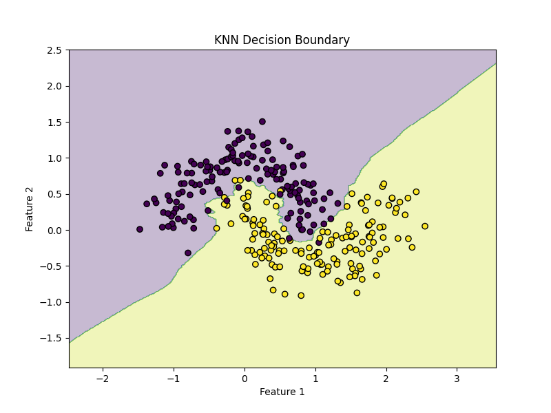
The make_moons dataset is very useful for understanding nonlinear decision boundaries.
import matplotlib.pyplot as plt

from sklearn.datasets import make_moons
from sklearn.model_selection import train_test_split
from sklearn.pipeline import Pipeline
from sklearn.preprocessing import StandardScaler
from sklearn.neighbors import KNeighborsClassifier

# Create nonlinear dataset
X, y = make_moons(n_samples=300, noise=0.2, random_state=42)

X_train, X_test, y_train, y_test = train_test_split(
    X, y, test_size=0.2, random_state=42
)

model = Pipeline([
    ("scaler", StandardScaler()),
    ("knn", KNeighborsClassifier(n_neighbors=5))
])

model.fit(X_train, y_train)

print("Accuracy:", model.score(X_test, y_test))
Plot the decision boundary
import numpy as np
import matplotlib.pyplot as plt

def plot_decision_boundary(model, X, y):
    x_min, x_max = X[:, 0].min() - 1, X[:, 0].max() + 1
    y_min, y_max = X[:, 1].min() - 1, X[:, 1].max() + 1

    xx, yy = np.meshgrid(
        np.linspace(x_min, x_max, 400),
        np.linspace(y_min, y_max, 400)
    )

    Z = model.predict(np.c_[xx.ravel(), yy.ravel()])
    Z = Z.reshape(xx.shape)

    plt.figure(figsize=(8, 6))
    plt.contourf(xx, yy, Z, alpha=0.3)
    plt.scatter(X[:, 0], X[:, 1], c=y, edgecolors="k")
    plt.title("KNN Decision Boundary")
    plt.xlabel("Feature 1")
    plt.ylabel("Feature 2")
    plt.show()

plot_decision_boundary(model, X, y)
KNN can create very flexible nonlinear boundaries because predictions depend on local neighborhoods rather than a global linear equation.
12) Effect of changing k
Try these values:
k = 1k = 5k = 15
for k in [1, 5, 15]:
    model = Pipeline([
        ("scaler", StandardScaler()),
        ("knn", KNeighborsClassifier(n_neighbors=k))
    ])
    model.fit(X_train, y_train)
    print(f"k={k}, accuracy={model.score(X_test, y_test):.4f}")
Interpretation
k=1often produces a very irregular boundary- medium
koften gives a better balance - large
kmakes the boundary smoother
Because n_neighbors directly controls how many nearby examples vote, it is one of the most important KNN hyperparameters.
Part III — Distance Weighting
13) Uniform vs distance weights
Scikit-learn provides a weights parameter in both classifier and regressor forms of KNN. Common choices are:
"uniform": all selected neighbors contribute equally"distance": closer neighbors contribute more
Example
from sklearn.pipeline import Pipeline
from sklearn.preprocessing import StandardScaler
from sklearn.neighbors import KNeighborsClassifier

uniform_model = Pipeline([
    ("scaler", StandardScaler()),
    ("knn", KNeighborsClassifier(n_neighbors=5, weights="uniform"))
])

distance_model = Pipeline([
    ("scaler", StandardScaler()),
    ("knn", KNeighborsClassifier(n_neighbors=5, weights="distance"))
])

uniform_model.fit(X_train, y_train)
distance_model.fit(X_train, y_train)

print("Uniform weights accuracy:", uniform_model.score(X_test, y_test))
print("Distance weights accuracy:", distance_model.score(X_test, y_test))
When distance weighting helps
Distance weighting can be useful when:
- close neighbors are much more informative than farther ones
- classes overlap
- you want less influence from more distant points inside the chosen
k
The scikit-learn nearest-neighbors classification example explicitly compares decision boundaries for different weights choices.
Part IV — Hyperparameter Tuning
14) Important KNN parameters
For KNeighborsClassifier and KNeighborsRegressor, the main parameters include:
n_neighborsweightsalgorithmleaf_sizepmetricn_jobs
Most important in practice
n_neighbors
How many neighbors to use.
weights
Whether neighbors all count equally or closer points count more.
p
Controls the Minkowski distance:
p=1→ Manhattanp=2→ Euclidean
metric
Distance function used by the model.
15) Tune KNN with GridSearchCV
from sklearn.model_selection import GridSearchCV
from sklearn.pipeline import Pipeline
from sklearn.preprocessing import StandardScaler
from sklearn.neighbors import KNeighborsClassifier

pipeline = Pipeline([
    ("scaler", StandardScaler()),
    ("knn", KNeighborsClassifier())
])

param_grid = {
    "knn__n_neighbors": [3, 5, 7, 9, 11, 15],
    "knn__weights": ["uniform", "distance"],
    "knn__p": [1, 2]
}

grid = GridSearchCV(
    estimator=pipeline,
    param_grid=param_grid,
    cv=5,
    scoring="accuracy",
    n_jobs=-1
)

grid.fit(X_train, y_train)

print("Best Parameters:", grid.best_params_)
print("Best CV Score:", grid.best_score_)

best_model = grid.best_estimator_
test_score = best_model.score(X_test, y_test)
print("Test Accuracy:", test_score)
What this does
It searches across:
- multiple
kvalues - different weighting strategies
- Manhattan vs Euclidean distance
This is the best practical way to find a strong KNN setup.
16) Why cross-validation matters
Choosing k based only on one train/test split can be unstable. Cross-validation gives a more reliable estimate by evaluating multiple folds of the training data. This is one of the core advantages of using scikit-learn’s model-selection tools together with pipelines.
Part V — KNN Regression
17) Example with KNeighborsRegressor
Now let us use KNN for regression.
import numpy as np
import matplotlib.pyplot as plt

from sklearn.neighbors import KNeighborsRegressor
from sklearn.model_selection import train_test_split
from sklearn.pipeline import Pipeline
from sklearn.preprocessing import StandardScaler
from sklearn.metrics import mean_squared_error, r2_score

# Synthetic data
rng = np.random.RandomState(42)
X = np.sort(5 * rng.rand(200, 1), axis=0)
y = np.sin(X).ravel()

# Add noise
y[::5] += 0.5 - rng.rand(40)

X_train, X_test, y_train, y_test = train_test_split(
    X, y, test_size=0.2, random_state=42
)

model = Pipeline([
    ("scaler", StandardScaler()),
    ("knn", KNeighborsRegressor(n_neighbors=5, weights="distance"))
])

model.fit(X_train, y_train)
y_pred = model.predict(X_test)

print("MSE:", mean_squared_error(y_test, y_pred))
print("R²:", r2_score(y_test, y_pred))
Plot predictions
X_plot = np.linspace(X.min(), X.max(), 500).reshape(-1, 1)
y_plot = model.predict(X_plot)

plt.figure(figsize=(8, 6))
plt.scatter(X, y, label="Data")
plt.plot(X_plot, y_plot, linewidth=2, label="KNN prediction")
plt.xlabel("X")
plt.ylabel("y")
plt.title("KNN Regression")
plt.legend()
plt.show()
KNeighborsRegressor predicts from nearby target values, and scikit-learn’s regression example shows this behavior for uniform and distance weighting.
18) Effect of k in regression
for k in [2, 5, 10, 20]:
    model = Pipeline([
        ("scaler", StandardScaler()),
        ("knn", KNeighborsRegressor(n_neighbors=k, weights="distance"))
    ])
    model.fit(X_train, y_train)
    y_pred = model.predict(X_test)
    print(f"k={k}, R²={r2_score(y_test, y_pred):.4f}")
Interpretation
- small
k: curve can become noisy - larger
k: curve becomes smoother - very large
k: model may become too flat
Part VI — A Full Real Workflow
19) End-to-end classification workflow
This is a solid real-project workflow for KNN.
Step 1: Load data
import pandas as pd

df = pd.read_csv("your_data.csv")
Step 2: Separate features and target
X = df.drop("target", axis=1)
y = df["target"]
Step 3: Split data
from sklearn.model_selection import train_test_split

X_train, X_test, y_train, y_test = train_test_split(
    X, y, test_size=0.2, random_state=42, stratify=y
)
Step 4: Build pipeline
from sklearn.pipeline import Pipeline
from sklearn.preprocessing import StandardScaler
from sklearn.neighbors import KNeighborsClassifier

pipeline = Pipeline([
    ("scaler", StandardScaler()),
    ("knn", KNeighborsClassifier())
])
Step 5: Tune parameters
from sklearn.model_selection import GridSearchCV

param_grid = {
    "knn__n_neighbors": [3, 5, 7, 9, 11, 15],
    "knn__weights": ["uniform", "distance"],
    "knn__p": [1, 2]
}

grid = GridSearchCV(
    pipeline,
    param_grid=param_grid,
    cv=5,
    scoring="accuracy",
    n_jobs=-1
)

grid.fit(X_train, y_train)
Step 6: Evaluate
from sklearn.metrics import classification_report, confusion_matrix, accuracy_score

best_model = grid.best_estimator_
y_pred = best_model.predict(X_test)

print("Best Params:", grid.best_params_)
print("Accuracy:", accuracy_score(y_test, y_pred))
print(confusion_matrix(y_test, y_pred))
print(classification_report(y_test, y_pred))
Step 7: Predict on new samples
new_samples = X_test.iloc[:5]
predictions = best_model.predict(new_samples)
print(predictions)
Part VII — How to Interpret Results
20) Classification metrics
For KNN classification, common metrics are:
- accuracy
- precision
- recall
- F1-score
- confusion matrix
If classes are balanced, accuracy can be informative. If classes are imbalanced, you should look beyond accuracy and inspect the full classification report.
from sklearn.metrics import confusion_matrix, classification_report

print(confusion_matrix(y_test, y_pred))
print(classification_report(y_test, y_pred))
21) Regression metrics
For KNN regression, common metrics are:
- MAE
- MSE
- RMSE
- R²
from sklearn.metrics import mean_absolute_error, mean_squared_error, r2_score
import numpy as np

mae = mean_absolute_error(y_test, y_pred)
mse = mean_squared_error(y_test, y_pred)
rmse = np.sqrt(mse)
r2 = r2_score(y_test, y_pred)

print("MAE:", mae)
print("MSE:", mse)
print("RMSE:", rmse)
print("R²:", r2)
Part VIII — Strengths and Weaknesses of KNN
22) Strengths
KNN is attractive because:
- it is simple to understand
- it works for classification and regression
- it can model nonlinear patterns
- it requires little explicit training
Since nearest-neighbors methods base predictions directly on nearby training examples, they can adapt well to local patterns without fitting a fixed global function.
23) Weaknesses
KNN also has important limitations:
- prediction can be slow on large datasets
- it is sensitive to scaling
- it can be hurt by irrelevant features
- performance depends strongly on
kand distance choice
Scikit-learn includes multiple nearest-neighbor search structures such as KDTree and BallTree, reflecting the fact that efficient neighbor lookup is an important practical concern in this family of algorithms.
Part IX — Common Mistakes
24) Not scaling the data
This is one of the biggest KNN mistakes.
Bad:
model = KNeighborsClassifier(n_neighbors=5)
model.fit(X_train, y_train)
Better:
model = Pipeline([
    ("scaler", StandardScaler()),
    ("knn", KNeighborsClassifier(n_neighbors=5))
])
Because KNN depends on distances, scaling can completely change which points count as nearest neighbors. StandardScaler and Pipeline are the standard scikit-learn tools for handling this correctly.
25) Choosing k arbitrarily
Do not choose k=5 just because it is the default.
Instead:
- try several
kvalues - use cross-validation
- compare metrics
The documented default is 5, but there is nothing magical about it; it is just a starting point.
26) Using too many irrelevant features
KNN can suffer badly when many features do not help, because they can distort distances. In practice, feature selection or dimensionality reduction may improve KNN performance.
27) Using KNN on very large datasets without thinking about cost
KNN may be easy to fit, but prediction can become expensive because the algorithm must compare new points to stored training examples. Scikit-learn exposes algorithm choices such as auto, and data structures like KDTree and BallTree, precisely because neighbor search efficiency matters.
Part X — Practical Advice
28) When should you use KNN?
Use KNN when:
- you want a simple baseline
- your dataset is small or medium-sized
- local similarity matters
- nonlinear boundaries are likely
It is often a good early model to compare against more advanced methods.
29) When should you avoid KNN?
Be careful with KNN when:
- the dataset is very large
- there are many irrelevant features
- the data is poorly scaled
- memory or prediction speed is a concern
30) A good default starting point
For classification:
Pipeline([
    ("scaler", StandardScaler()),
    ("knn", KNeighborsClassifier(n_neighbors=5, weights="distance"))
])
For regression:
Pipeline([
    ("scaler", StandardScaler()),
    ("knn", KNeighborsRegressor(n_neighbors=5, weights="distance"))
])
This is a strong starting point because:
- scaling protects the distance calculations
weights="distance"often improves local sensitivityk=5is a reasonable baseline to tune from
The estimator defaults and options for weights, metric, p, and n_neighbors are documented in the current scikit-learn API.
Part XI — Mini Project Example
31) Predicting flower species with KNN
Here is a compact but realistic mini-project using Iris.
from sklearn.datasets import load_iris
from sklearn.model_selection import train_test_split, GridSearchCV
from sklearn.pipeline import Pipeline
from sklearn.preprocessing import StandardScaler
from sklearn.neighbors import KNeighborsClassifier
from sklearn.metrics import classification_report, confusion_matrix, accuracy_score

# Load
data = load_iris()
X, y = data.data, data.target

# Split
X_train, X_test, y_train, y_test = train_test_split(
    X, y, test_size=0.2, stratify=y, random_state=42
)

# Pipeline
pipeline = Pipeline([
    ("scaler", StandardScaler()),
    ("knn", KNeighborsClassifier())
])

# Search space
param_grid = {
    "knn__n_neighbors": [3, 5, 7, 9, 11],
    "knn__weights": ["uniform", "distance"],
    "knn__p": [1, 2]
}

# Grid search
grid = GridSearchCV(
    pipeline,
    param_grid=param_grid,
    cv=5,
    scoring="accuracy",
    n_jobs=-1
)

grid.fit(X_train, y_train)

# Evaluate
best_model = grid.best_estimator_
y_pred = best_model.predict(X_test)

print("Best Parameters:", grid.best_params_)
print("Accuracy:", accuracy_score(y_test, y_pred))
print("\nConfusion Matrix:\n", confusion_matrix(y_test, y_pred))
print("\nClassification Report:\n", classification_report(y_test, y_pred))
Why this project is good
- uses train/test split
- scales correctly
- tunes
k, weights, and distance behavior - evaluates only on the held-out test set
Part XII — Summary
32) What you should remember
KNN is one of the easiest machine learning algorithms to understand.
The central idea is:
- look at nearby examples
- use them to predict the label or value of a new point
For KNN classification, neighbors vote.
For KNN regression, neighbors contribute numeric values.
The most important practical rules are:
- always scale features
- tune
n_neighbors - compare uniform vs distance weights
- experiment with Manhattan and Euclidean distance
- use cross-validation
- be careful on large datasets
These recommendations are fully consistent with the current scikit-learn nearest-neighbors, preprocessing, and pipeline documentation.
33) Final ready-to-use template
from sklearn.model_selection import train_test_split, GridSearchCV
from sklearn.pipeline import Pipeline
from sklearn.preprocessing import StandardScaler
from sklearn.neighbors import KNeighborsClassifier
from sklearn.metrics import classification_report

# X, y = your data

X_train, X_test, y_train, y_test = train_test_split(
    X, y, test_size=0.2, random_state=42
)

pipeline = Pipeline([
    ("scaler", StandardScaler()),
    ("knn", KNeighborsClassifier())
])

param_grid = {
    "knn__n_neighbors": [3, 5, 7, 9, 11, 15],
    "knn__weights": ["uniform", "distance"],
    "knn__p": [1, 2]
}

grid = GridSearchCV(
    pipeline,
    param_grid=param_grid,
    cv=5,
    scoring="accuracy",
    n_jobs=-1
)

grid.fit(X_train, y_train)

print("Best params:", grid.best_params_)
print("Test score:", grid.best_estimator_.score(X_test, y_test))

y_pred = grid.best_estimator_.predict(X_test)
print(classification_report(y_test, y_pred))
34) Practice exercises
Exercise 1
Train a KNN classifier on the Iris dataset and report accuracy.
Exercise 2
Train KNN on make_moons and visualize the decision boundary.
Exercise 3
Tune n_neighbors, weights, and p using GridSearchCV.
Exercise 4
Compare weights="uniform" and weights="distance".
Exercise 5
Train a KNeighborsRegressor model on a nonlinear synthetic regression dataset.
Final summary
What each exercise teaches
- Exercise 1: basic KNN classification
- Exercise 2: nonlinear classification and visualization
- Exercise 3: hyperparameter tuning
- Exercise 4: comparison of weight strategies
- Exercise 5: nonlinear regression with KNN









💬 Comments
No comments yet. Be the first to comment!
Login to comment.