
0) Introduction
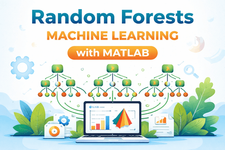
Random Forests are supervised machine learning algorithms used for both classification and regression. In scikit-learn, the main classes are RandomForestClassifier and RandomForestRegressor. A random forest is a meta-estimator that fits many decision trees on different subsamples of the data and uses averaging to improve predictive accuracy and reduce overfitting compared with a single tree.
1) What a Random Forest does
A Random Forest builds many decision trees instead of relying on just one.
For classification:
- each tree predicts a class
- the forest combines the trees by voting
- the final class is the majority vote
For regression:
- each tree predicts a number
- the forest averages those predictions
- the final prediction is the average
This averaging is the main reason Random Forests are usually more stable and more accurate than a single decision tree. Scikit-learn explicitly describes random forests as ensembles that use averaging to improve predictive accuracy and control overfitting.
2) Why Random Forests are useful
Random Forests are popular because they are:
- powerful on tabular data
- less likely to overfit than a single tree
- usable for both classification and regression
- able to model nonlinear patterns
- not very sensitive to feature scaling
They are often a strong baseline for many practical machine learning problems. They belong to scikit-learn’s ensemble methods family, which combines multiple predictors to improve robustness and generalization.
3) Why it is called “Random Forest”
The method is “random” for two main reasons.
1. Random sampling of training data
Each tree is trained on a different subsample of the data. In scikit-learn, this is controlled by bootstrap=True by default, and the sub-sample size can also be controlled with max_samples.
2. Random subset of features
At each split, the tree considers only a subset of features rather than all of them. This randomness helps the trees become less correlated with each other, which improves the ensemble effect. The main control for this is max_features.
So the forest becomes strong because:
- each tree is different
- the errors of individual trees are less correlated
- averaging reduces variance
4) Random Forest vs Decision Tree
A Decision Tree is one tree.
A Random Forest is many trees combined together.
A single Decision Tree
- easy to interpret
- can overfit easily
- unstable to small data changes
A Random Forest
- harder to interpret directly
- usually more accurate
- more robust and stable
- less likely to overfit than one tree
Scikit-learn’s documentation emphasizes that random forests improve predictive accuracy and control overfitting by averaging many trees.
5) Why Random Forests usually do not need feature scaling
Random Forests are based on decision trees, and trees split on thresholds such as:
feature <= valuefeature > value
They do not rely on geometric distances like KNN or margin geometry like SVM. Because of this, feature scaling is usually not necessary for Random Forests. This follows from the tree-based structure described in scikit-learn’s ensemble and tree documentation.
That is one of the practical advantages of tree-based models.
Part I — First Classification Example
6) Install required libraries
pip install numpy pandas matplotlib scikit-learn7) A simple Random Forest classification example
We will use the Breast Cancer dataset from scikit-learn.
import numpy as np
import pandas as pd

from sklearn.datasets import load_breast_cancer
from sklearn.model_selection import train_test_split
from sklearn.ensemble import RandomForestClassifier
from sklearn.metrics import accuracy_score, classification_report, confusion_matrix

# Load dataset
data = load_breast_cancer()
X = data.data
y = data.target

# Split
X_train, X_test, y_train, y_test = train_test_split(
    X, y, test_size=0.2, random_state=42, stratify=y
)

# Build model
model = RandomForestClassifier(
    n_estimators=100,
    random_state=42
)

# Train
model.fit(X_train, y_train)

# Predict
y_pred = model.predict(X_test)

# Evaluate
print("Accuracy:", accuracy_score(y_test, y_pred))
print("\nConfusion Matrix:\n", confusion_matrix(y_test, y_pred))
print("\nClassification Report:\n", classification_report(y_test, y_pred))
What this code does
- loads the dataset
- splits it into train and test sets
- trains a forest with 100 trees
- predicts on the test set
- evaluates the model
In scikit-learn, n_estimators is the number of trees in the forest, and RandomForestClassifier fits multiple decision tree classifiers on different sub-samples of the dataset.
8) Predicting class probabilities
Random Forests can also output probabilities with predict_proba.
proba = model.predict_proba(X_test[:5])
print(proba)
For classification, the forest combines information from its trees to produce class probabilities and class predictions. The classifier API in scikit-learn includes predict, predict_proba, and score.
Part II — Important Parameters
9) Key parameters for RandomForestClassifier
Important parameters include:
n_estimatorscriterionmax_depthmin_samples_splitmin_samples_leafmax_featuresbootstrapmax_samplesoob_scoren_jobsrandom_stateclass_weight
n_estimators
Number of trees in the forest.
- small value → faster but less stable
- larger value → more stable predictions but slower training
max_depth
Maximum depth of each tree.
- smaller depth → simpler trees
- larger depth → more complex trees
max_features
Number of features considered at each split.
This is one of the key sources of randomness in the forest.
bootstrap
Whether each tree is trained on a bootstrap sample. Default is True.
oob_score
Whether to use out-of-bag samples for validation. This is only available when bootstrapping is enabled.
10) What is out-of-bag evaluation
When bootstrap sampling is used, each tree is trained on a sample drawn with replacement from the training set. That means some training points are left out for that tree. These are called out-of-bag samples.
You can use them to estimate performance without needing a separate validation set for every tree.
model = RandomForestClassifier(
    n_estimators=200,
    oob_score=True,
    random_state=42
)

model.fit(X_train, y_train)
print("OOB Score:", model.oob_score_)
Scikit-learn exposes oob_score directly in the Random Forest API when bootstrapping is enabled.
Part III — Why Random Forests work well
11) Bagging intuition
Random Forests are a form of bagging.
Bagging means:
- train many models on different bootstrap samples
- average the predictions
Averaging reduces variance. This is especially helpful for decision trees because single trees can vary a lot from one sample to another. Random forests add extra randomness through feature subsampling on top of bagging.
12) Why more trees usually help
In a Random Forest:
- one bad tree is not a disaster
- noisy trees can be corrected by the others
- more trees usually make predictions more stable
Adding trees usually helps until performance levels off, though training and prediction become slower. n_estimators is therefore one of the most important practical controls in scikit-learn’s API.
Part IV — Feature Importance
13) Built-in feature importance
Random Forests in scikit-learn expose feature_importances_.
import pandas as pd

importance = pd.Series(model.feature_importances_, index=data.feature_names)
print(importance.sort_values(ascending=False))
Scikit-learn’s forest importance example shows how a forest of trees can be used to evaluate feature importance, and it also visualizes variability across trees.
Why this is useful
Feature importance helps you understand which variables the forest relied on the most.
14) Plot feature importance
import matplotlib.pyplot as plt

importance = importance.sort_values(ascending=True)

plt.figure(figsize=(8, 6))
importance.plot(kind="barh")
plt.title("Random Forest Feature Importance")
plt.xlabel("Importance")
plt.ylabel("Feature")
plt.show()
The scikit-learn example on forest importances uses impurity-based importances and shows inter-tree variability with error bars.
15) Important caution about feature importance
Scikit-learn also provides an example comparing impurity-based Random Forest importances with permutation importance, and it warns that impurity-based importance can inflate the importance of numerical features in some settings.
So built-in feature importance is useful, but it should be interpreted carefully.
Permutation importance example
from sklearn.inspection import permutation_importance

result = permutation_importance(
    model, X_test, y_test, n_repeats=10, random_state=42, n_jobs=-1
)

perm_importance = pd.Series(result.importances_mean, index=data.feature_names)
print(perm_importance.sort_values(ascending=False))
Permutation importance is often a better diagnostic when you want a more reliable picture of feature influence. This is an inference grounded in scikit-learn’s comparison example.
Part V — Tuning a Random Forest
16) Tune with GridSearchCV
from sklearn.model_selection import GridSearchCV
from sklearn.ensemble import RandomForestClassifier

param_grid = {
    "n_estimators": [100, 200, 300],
    "max_depth": [None, 5, 10, 20],
    "min_samples_split": [2, 5, 10],
    "min_samples_leaf": [1, 2, 4],
    "max_features": ["sqrt", "log2"]
}

grid = GridSearchCV(
    estimator=RandomForestClassifier(random_state=42),
    param_grid=param_grid,
    cv=5,
    scoring="accuracy",
    n_jobs=-1
)

grid.fit(X_train, y_train)

print("Best Parameters:", grid.best_params_)
print("Best CV Score:", grid.best_score_)

best_model = grid.best_estimator_
y_pred = best_model.predict(X_test)
print("Test Accuracy:", accuracy_score(y_test, y_pred))
Why this helps
Instead of guessing the best forest size or depth, you let cross-validation search for a stronger combination.
The most influential tuning parameters in practice are usually:
n_estimatorsmax_depthmin_samples_splitmin_samples_leafmax_features
17) A good practical starting point
A strong default starting point for classification is often something like:
model = RandomForestClassifier(
    n_estimators=200,
    max_depth=None,
    min_samples_split=2,
    min_samples_leaf=1,
    max_features="sqrt",
    random_state=42,
    n_jobs=-1
)
This is not universally optimal, but it is a sensible baseline built from the core parameters exposed in the current scikit-learn API.
Part VI — Random Forest Regression
18) Example with RandomForestRegressor
Now let us use a Random Forest for regression.
import numpy as np
import matplotlib.pyplot as plt

from sklearn.ensemble import RandomForestRegressor
from sklearn.model_selection import train_test_split
from sklearn.metrics import mean_squared_error, r2_score

# Synthetic data
rng = np.random.RandomState(42)
X = np.sort(5 * rng.rand(200, 1), axis=0)
y = np.sin(X).ravel()

# Add noise
y[::5] += 0.5 - rng.rand(40)

X_train, X_test, y_train, y_test = train_test_split(
    X, y, test_size=0.2, random_state=42
)

model = RandomForestRegressor(
    n_estimators=200,
    random_state=42
)

model.fit(X_train, y_train)
y_pred = model.predict(X_test)

print("MSE:", mean_squared_error(y_test, y_pred))
print("R²:", r2_score(y_test, y_pred))
Scikit-learn defines RandomForestRegressor analogously to the classifier: it fits many decision tree regressors on different subsamples and uses averaging to improve predictive accuracy and control overfitting.
19) Plot regression predictions
X_plot = np.linspace(X.min(), X.max(), 500).reshape(-1, 1)
y_plot = model.predict(X_plot)

plt.figure(figsize=(8, 6))
plt.scatter(X, y, label="Data")
plt.plot(X_plot, y_plot, linewidth=2, label="Random Forest prediction")
plt.xlabel("X")
plt.ylabel("y")
plt.title("Random Forest Regression")
plt.legend()
plt.show()
Random Forest regression often gives smoother and more robust predictions than a single decision tree regressor because it averages many trees. That is an inference directly supported by the ensemble definition in the scikit-learn API.
20) Important regression parameters
RandomForestRegressor shares many structural parameters with the classifier version, including:
n_estimatorscriterionmax_depthmin_samples_splitmin_samples_leafmax_featuresbootstrapmax_samplesoob_scoren_jobs
Example:
model = RandomForestRegressor(
    n_estimators=300,
    max_depth=10,
    min_samples_leaf=2,
    random_state=42,
    n_jobs=-1
)
Part VII — A Full Real Workflow
21) End-to-end classification workflow
Step 1: Load data
import pandas as pd

df = pd.read_csv("your_data.csv")
Step 2: Separate features and target
X = df.drop("target", axis=1)
y = df["target"]
Step 3: Split data
from sklearn.model_selection import train_test_split

X_train, X_test, y_train, y_test = train_test_split(
    X, y, test_size=0.2, random_state=42, stratify=y
)
Step 4: Build model
from sklearn.ensemble import RandomForestClassifier

model = RandomForestClassifier(random_state=42)
Step 5: Tune parameters
from sklearn.model_selection import GridSearchCV

param_grid = {
    "n_estimators": [100, 200],
    "max_depth": [None, 5, 10],
    "min_samples_split": [2, 5, 10],
    "min_samples_leaf": [1, 2, 4],
    "max_features": ["sqrt", "log2"]
}

grid = GridSearchCV(
    model,
    param_grid=param_grid,
    cv=5,
    scoring="accuracy",
    n_jobs=-1
)

grid.fit(X_train, y_train)
Step 6: Evaluate
from sklearn.metrics import classification_report, confusion_matrix, accuracy_score

best_model = grid.best_estimator_
y_pred = best_model.predict(X_test)

print("Best Params:", grid.best_params_)
print("Accuracy:", accuracy_score(y_test, y_pred))
print(confusion_matrix(y_test, y_pred))
print(classification_report(y_test, y_pred))
Step 7: Predict on new samples
new_samples = X_test.iloc[:5]
predictions = best_model.predict(new_samples)
print(predictions)
This workflow follows scikit-learn’s standard estimator and model selection pattern for ensemble estimators.
Part VIII — How to Read the Results
22) Classification metrics
For classification, common metrics are:
- accuracy
- precision
- recall
- F1-score
- confusion matrix
from sklearn.metrics import confusion_matrix, classification_report

print(confusion_matrix(y_test, y_pred))
print(classification_report(y_test, y_pred))
Random forests support binary and multiclass classification through the same RandomForestClassifier API.
23) Regression metrics
For regression, common metrics are:
- MAE
- MSE
- RMSE
- R²
from sklearn.metrics import mean_absolute_error, mean_squared_error, r2_score
import numpy as np

mae = mean_absolute_error(y_test, y_pred)
mse = mean_squared_error(y_test, y_pred)
rmse = np.sqrt(mse)
r2 = r2_score(y_test, y_pred)

print("MAE:", mae)
print("MSE:", mse)
print("RMSE:", rmse)
print("R²:", r2)
Random forest regressors also support multi-output regression natively, as shown in scikit-learn’s example comparing random forest regression with a multi-output meta-estimator.
Part IX — Strengths and Weaknesses
24) Strengths of Random Forests
Random Forests are strong because they are:
- usually more accurate than a single decision tree
- robust to overfitting compared with one tree
- good at modeling nonlinear relationships
- useful without feature scaling
- able to provide feature importance estimates
These strengths follow directly from scikit-learn’s description of random forests as ensembles of trees that improve predictive accuracy and control overfitting.
25) Weaknesses of Random Forests
They also have limitations:
- less interpretable than a single decision tree
- can be slower than one tree
- large forests use more memory
- impurity-based feature importance can be misleading in some cases
Scikit-learn’s comparison examples also show that computation time matters when comparing forest methods with alternatives such as Histogram Gradient Boosting.
Part X — Common Mistakes
26) Using too few trees
Bad:
model = RandomForestClassifier(n_estimators=10, random_state=42)This may work, but the predictions can be less stable.
Better:
model = RandomForestClassifier(n_estimators=200, random_state=42, n_jobs=-1)Because the forest prediction is an average across trees, too few trees can leave performance unnecessarily noisy. This is a practical inference grounded in the ensemble formulation.
27) Ignoring max_depth and leaf controls
Even though Random Forests reduce overfitting compared with a single tree, forests can still become unnecessarily complex.
Good parameters to tune:
max_depthmin_samples_splitmin_samples_leafmax_features
28) Treating built-in feature importance as absolute truth
Impurity-based importance is convenient, but scikit-learn’s permutation importance comparison shows it can overstate the importance of some feature types. Use it carefully, and compare with permutation importance when interpretability matters.
Part XI — Practical Advice
29) When should you use Random Forests?
Use Random Forests when:
- you want a strong tabular-data baseline
- you expect nonlinear relationships
- you want something robust and practical
- interpretability of a single rule tree is not your top priority
30) When should you avoid them?
Be careful with Random Forests when:
- you need maximum interpretability
- you need very fast lightweight models
- your dataset is extremely large and training cost matters a lot
In those cases, simpler models or other ensemble methods may be worth comparing. Scikit-learn’s ensemble examples include comparisons with Histogram Gradient Boosting specifically on score and computation time.
31) A good default starting point
For classification:
RandomForestClassifier(
    n_estimators=200,
    max_features="sqrt",
    random_state=42,
    n_jobs=-1
)
For regression:
RandomForestRegressor(
    n_estimators=200,
    max_features=1.0,
    random_state=42,
    n_jobs=-1
)
These are sensible baseline starting points based on the current parameterized API for the stable scikit-learn random forest estimators.
Part XII — Mini Project Example
32) Predicting iris species with a Random Forest
from sklearn.datasets import load_iris
from sklearn.model_selection import train_test_split, GridSearchCV
from sklearn.ensemble import RandomForestClassifier
from sklearn.metrics import classification_report, confusion_matrix, accuracy_score

# Load
data = load_iris()
X, y = data.data, data.target

# Split
X_train, X_test, y_train, y_test = train_test_split(
    X, y, test_size=0.2, stratify=y, random_state=42
)

# Model
model = RandomForestClassifier(random_state=42)

# Search space
param_grid = {
    "n_estimators": [100, 200, 300],
    "max_depth": [None, 3, 5, 10],
    "min_samples_split": [2, 5, 10],
    "min_samples_leaf": [1, 2, 4],
    "max_features": ["sqrt", "log2"]
}

# Grid search
grid = GridSearchCV(
    model,
    param_grid=param_grid,
    cv=5,
    scoring="accuracy",
    n_jobs=-1
)

grid.fit(X_train, y_train)

# Evaluate
best_model = grid.best_estimator_
y_pred = best_model.predict(X_test)

print("Best Parameters:", grid.best_params_)
print("Accuracy:", accuracy_score(y_test, y_pred))
print("\nConfusion Matrix:\n", confusion_matrix(y_test, y_pred))
print("\nClassification Report:\n", classification_report(y_test, y_pred))
Why this mini-project is good
- uses a train/test split
- tunes the most important forest parameters
- evaluates on held-out data
- stays close to real practice
This matches scikit-learn’s general estimator, ensemble, and cross-validation workflow.
Part XIII — Summary
33) What you should remember
Random Forests are one of the most practical and powerful classical machine learning algorithms.
The core idea is:
- train many decision trees
- make them different through randomness
- combine their predictions by voting or averaging
For classification, they vote.
For regression, they average.
This improves predictive accuracy and helps control overfitting compared with a single decision tree.
The most important practical rules are:
- feature scaling is usually not needed
- tune
n_estimators - tune
max_depth,min_samples_split, andmin_samples_leaf - tune
max_features - use cross-validation
- interpret built-in feature importance carefully
These recommendations align with the current scikit-learn Random Forest API, user guide, and feature-importance examples.
34) Final ready-to-use template
from sklearn.model_selection import train_test_split, GridSearchCV
from sklearn.ensemble import RandomForestClassifier
from sklearn.metrics import classification_report

# X, y = your data

X_train, X_test, y_train, y_test = train_test_split(
    X, y, test_size=0.2, random_state=42
)

model = RandomForestClassifier(random_state=42)

param_grid = {
    "n_estimators": [100, 200],
    "max_depth": [None, 5, 10],
    "min_samples_split": [2, 5, 10],
    "min_samples_leaf": [1, 2, 4],
    "max_features": ["sqrt", "log2"]
}

grid = GridSearchCV(
    model,
    param_grid=param_grid,
    cv=5,
    scoring="accuracy",
    n_jobs=-1
)

grid.fit(X_train, y_train)

print("Best params:", grid.best_params_)
print("Test score:", grid.best_estimator_.score(X_test, y_test))

y_pred = grid.best_estimator_.predict(X_test)
print(classification_report(y_test, y_pred))
35) Practice exercises
Exercise 1
Train a RandomForestClassifier on the Iris dataset and report accuracy.
Exercise 2
Train a Random Forest on the Breast Cancer dataset and display feature importances.
Exercise 3
Tune n_estimators, max_depth, and max_features using GridSearchCV.
Exercise 4
Compare a single DecisionTreeClassifier with a RandomForestClassifier.
Exercise 5
Train a RandomForestRegressor on a nonlinear synthetic regression dataset.
Final summary
What each exercise teaches
- Exercise 1: basic Random Forest classification
- Exercise 2: feature importance analysis
- Exercise 3: hyperparameter tuning
- Exercise 4: comparison between a single tree and a forest
- Exercise 5: nonlinear regression with Random Forest










💬 Comments
No comments yet. Be the first to comment!
Login to comment.