
0) Introduction
Gradient Boosting is a supervised machine learning technique used for both classification and regression. In scikit-learn, the main estimators are GradientBoostingClassifier and GradientBoostingRegressor. These models build an additive ensemble in a forward, stage-wise way, where each new tree is trained to improve the errors of the current ensemble. Scikit-learn describes this as fitting regression trees on the negative gradient of the loss function.
1) What Gradient Boosting does
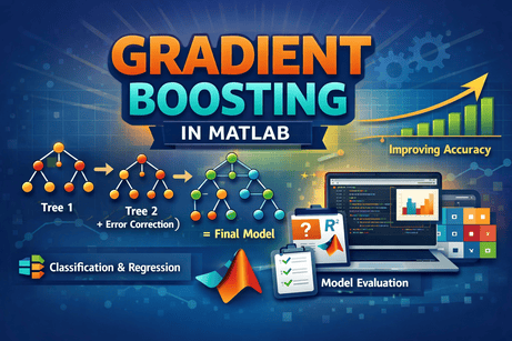
A Gradient Boosting model builds many small decision trees, but unlike Random Forests, it does not train them independently.
Instead, it works sequentially:
- build a first weak tree
- measure the current errors
- build a new tree to correct those errors
- repeat many times
So the model improves step by step.
That is the central idea:
- weak learners: usually small decision trees
- boosting: each new tree focuses on correcting previous mistakes
- additive model: predictions are built by summing the contributions of many trees
Scikit-learn states that Gradient Boosting builds an additive model in a forward stage-wise fashion and optimizes differentiable loss functions.
2) Why Gradient Boosting is powerful
Gradient Boosting is popular because it often performs very well on structured/tabular data.
It is useful when:
- relationships are nonlinear
- features interact in complex ways
- you want stronger predictive performance than a single tree
- you want a classical model that is often very competitive
Scikit-learn also documents histogram-based gradient boosting estimators, HistGradientBoostingClassifier and HistGradientBoostingRegressor, as much faster variants for larger datasets, especially when the number of samples is around 10,000 or more.
3) Gradient Boosting vs Random Forest
These two methods both use trees, but they work differently.
Random Forest
- trains many trees independently
- combines them by averaging or voting
- mainly reduces variance
Gradient Boosting
- trains trees sequentially
- each tree corrects previous errors
- mainly reduces bias, while regularization helps control variance
This difference is reflected in scikit-learn’s descriptions: Random Forests average many trees, while Gradient Boosting adds trees stage by stage based on loss gradients.
4) The idea of weak learners
In Gradient Boosting, the trees are usually small.
Typical settings:
- shallow trees
- limited depth
- each tree captures only a small pattern
Why?
Because one very large tree could overfit quickly. Boosting instead combines many small corrections into a strong final model.
This is why max_depth and related tree controls are important in gradient boosting models. Scikit-learn’s regression example demonstrates using 500 regression trees of depth 4 and shows how boosting builds predictive strength from many such trees.
5) Learning rate intuition
One of the most important parameters is learning_rate.
It controls how much each new tree contributes.
- small learning rate: slower learning, often better generalization, usually needs more trees
- large learning rate: faster learning, but higher overfitting risk
Scikit-learn’s regularization example explicitly notes that shrinkage with learning_rate < 1.0 improves performance considerably, and that it works especially well with stochastic boosting.
6) Number of trees: n_estimators
Another important parameter is n_estimators.
This is the number of boosting stages, meaning the number of trees added to the model.
- too few trees → underfitting
- too many trees → can overfit, especially without enough regularization
The balance between learning_rate and n_estimators is one of the most important practical tuning choices in Gradient Boosting. This follows directly from the stage-wise additive formulation in scikit-learn’s estimators and regularization examples.
7) Do Gradient Boosting models need feature scaling?
Like other tree-based models, classical Gradient Boosting with decision trees usually does not require feature scaling, because splits are based on thresholds on individual features rather than geometric distances. This is an inference from the fact that these estimators are tree ensembles in scikit-learn’s ensemble module.
That means you usually do not need StandardScaler here.
Part I — First Classification Example
8) Install required libraries
pip install numpy pandas matplotlib scikit-learn9) A simple Gradient Boosting classification example
We will use the Breast Cancer dataset from scikit-learn.
import numpy as np
import pandas as pd

from sklearn.datasets import load_breast_cancer
from sklearn.model_selection import train_test_split
from sklearn.ensemble import GradientBoostingClassifier
from sklearn.metrics import accuracy_score, classification_report, confusion_matrix

# Load dataset
data = load_breast_cancer()
X = data.data
y = data.target

# Split
X_train, X_test, y_train, y_test = train_test_split(
    X, y, test_size=0.2, random_state=42, stratify=y
)

# Build model
model = GradientBoostingClassifier(
    n_estimators=100,
    learning_rate=0.1,
    max_depth=3,
    random_state=42
)

# Train
model.fit(X_train, y_train)

# Predict
y_pred = model.predict(X_test)

# Evaluate
print("Accuracy:", accuracy_score(y_test, y_pred))
print("\nConfusion Matrix:\n", confusion_matrix(y_test, y_pred))
print("\nClassification Report:\n", classification_report(y_test, y_pred))
What this code does
- loads the dataset
- splits it into train and test sets
- trains a gradient boosting classifier
- predicts on the test set
- evaluates performance
GradientBoostingClassifier builds an additive model stage by stage and, for classification, fits regression trees to the negative gradient of the classification loss.
10) Predicting class probabilities
Gradient Boosting can also output probabilities.
proba = model.predict_proba(X_test[:5])
print(proba)
The classifier API in scikit-learn supports probability prediction for gradient boosting classification.
Part II — Important Parameters
11) Key parameters for GradientBoostingClassifier
Important parameters include:
losslearning_raten_estimatorssubsamplecriterionmax_depthmin_samples_splitmin_samples_leafmax_featuresvalidation_fractionn_iter_no_changetolrandom_state
learning_rate
Controls how much each tree contributes.
n_estimators
Number of boosting stages.
subsample
Fraction of samples used to fit each base learner.
If subsample < 1.0, you get stochastic gradient boosting, which scikit-learn notes can reduce variance when combined with shrinkage.
max_depth
Controls the depth of each individual regression tree used in boosting.
max_features
Controls the number of features considered when looking for the best split, and scikit-learn notes this can reduce variance similarly to random feature subsampling in Random Forests.
12) Early stopping
Scikit-learn supports early stopping for classical Gradient Boosting through parameters like:
validation_fractionn_iter_no_changetol
This means the training can stop automatically if validation performance stops improving.
Example:
from sklearn.ensemble import GradientBoostingClassifier

model = GradientBoostingClassifier(
    n_estimators=500,
    learning_rate=0.05,
    max_depth=3,
    validation_fraction=0.1,
    n_iter_no_change=10,
    tol=1e-4,
    random_state=42
)

model.fit(X_train, y_train)
print("Used estimators:", model.n_estimators_)
This helps avoid training too long and overfitting.
Part III — Regularization in Gradient Boosting
13) The main ways to regularize the model
Gradient Boosting can overfit if left uncontrolled. Common ways to regularize it include:
- reducing
learning_rate - limiting
max_depth - increasing
min_samples_leaf - using
subsample < 1.0 - using early stopping
Scikit-learn’s regularization example highlights shrinkage and stochastic gradient boosting as key regularization tools.
14) A regularized example
model = GradientBoostingClassifier(
    n_estimators=300,
    learning_rate=0.05,
    max_depth=2,
    min_samples_leaf=5,
    subsample=0.8,
    random_state=42
)
Why this helps:
- smaller trees reduce complexity
- smaller learning rate makes updates gentler
- subsampling adds randomness and can reduce variance
- larger leaves reduce sensitivity to noise
These choices reflect the regularization mechanisms documented in scikit-learn’s gradient boosting examples.
Part IV — Tuning a Gradient Boosting Classifier
15) Tune with GridSearchCV
from sklearn.model_selection import GridSearchCV
from sklearn.ensemble import GradientBoostingClassifier

param_grid = {
    "n_estimators": [100, 200, 300],
    "learning_rate": [0.01, 0.05, 0.1],
    "max_depth": [2, 3, 4],
    "min_samples_leaf": [1, 3, 5],
    "subsample": [0.8, 1.0]
}

grid = GridSearchCV(
    estimator=GradientBoostingClassifier(random_state=42),
    param_grid=param_grid,
    cv=5,
    scoring="accuracy",
    n_jobs=-1
)

grid.fit(X_train, y_train)

print("Best Parameters:", grid.best_params_)
print("Best CV Score:", grid.best_score_)

best_model = grid.best_estimator_
y_pred = best_model.predict(X_test)
print("Test Accuracy:", accuracy_score(y_test, y_pred))
Most important tuning parameters in practice
The most important ones are usually:
learning_raten_estimatorsmax_depthsubsamplemin_samples_leaf
That follows from scikit-learn’s API and regularization guidance for gradient boosting.
Part V — Feature Importance
16) Built-in feature importance
Like other tree ensembles, Gradient Boosting models expose feature_importances_.
import pandas as pd

importance = pd.Series(model.feature_importances_, index=data.feature_names)
print(importance.sort_values(ascending=False))
These are impurity-based importances derived from the boosted trees. This is supported by the estimator APIs in scikit-learn.
17) Plot feature importance
import matplotlib.pyplot as plt

importance = importance.sort_values(ascending=True)

plt.figure(figsize=(8, 6))
importance.plot(kind="barh")
plt.title("Gradient Boosting Feature Importance")
plt.xlabel("Importance")
plt.ylabel("Feature")
plt.show()
Caution
As with other tree ensembles, impurity-based importances can be misleading in some settings. Scikit-learn’s permutation-importance comparison warns about this issue for tree-based models.
A more robust diagnostic is often permutation importance:
from sklearn.inspection import permutation_importance

result = permutation_importance(
    model, X_test, y_test, n_repeats=10, random_state=42, n_jobs=-1
)

perm_importance = pd.Series(result.importances_mean, index=data.feature_names)
print(perm_importance.sort_values(ascending=False))
Part VI — Gradient Boosting Regression
18) Example with GradientBoostingRegressor
Now let us use Gradient Boosting for regression.
import numpy as np
import matplotlib.pyplot as plt

from sklearn.ensemble import GradientBoostingRegressor
from sklearn.model_selection import train_test_split
from sklearn.metrics import mean_squared_error, r2_score

# Synthetic data
rng = np.random.RandomState(42)
X = np.sort(5 * rng.rand(200, 1), axis=0)
y = np.sin(X).ravel()

# Add noise
y[::5] += 0.5 - rng.rand(40)

X_train, X_test, y_train, y_test = train_test_split(
    X, y, test_size=0.2, random_state=42
)

model = GradientBoostingRegressor(
    n_estimators=300,
    learning_rate=0.05,
    max_depth=3,
    random_state=42
)

model.fit(X_train, y_train)
y_pred = model.predict(X_test)

print("MSE:", mean_squared_error(y_test, y_pred))
print("R²:", r2_score(y_test, y_pred))
Scikit-learn documents GradientBoostingRegressor as a stage-wise additive model that fits regression trees on the negative gradient of the loss, and notes that HistGradientBoostingRegressor is a much faster variant for intermediate and large datasets.
19) Plot regression predictions
X_plot = np.linspace(X.min(), X.max(), 500).reshape(-1, 1)
y_plot = model.predict(X_plot)

plt.figure(figsize=(8, 6))
plt.scatter(X, y, label="Data")
plt.plot(X_plot, y_plot, linewidth=2, label="Gradient Boosting prediction")
plt.xlabel("X")
plt.ylabel("y")
plt.title("Gradient Boosting Regression")
plt.legend()
plt.show()
Scikit-learn’s official regression example uses Gradient Boosting to solve a regression task and illustrates this type of boosted predictive fit.
20) Important regression parameters
For GradientBoostingRegressor, the important parameters are very similar:
losslearning_raten_estimatorssubsamplecriterionmax_depthmin_samples_splitmin_samples_leafmax_featuresvalidation_fractionn_iter_no_changetol
Scikit-learn also notes that gradient boosting regression supports different regression losses, and modern names include squared_error, with older aliases deprecated.
Part VII — Histogram Gradient Boosting
21) What is Histogram Gradient Boosting?
Scikit-learn provides:
HistGradientBoostingClassifierHistGradientBoostingRegressor
These are histogram-based gradient boosting estimators.
Scikit-learn states they are much faster than the classical gradient boosting estimators on large datasets, particularly when n_samples >= 10,000. It also notes they were inspired by LightGBM.
When to prefer them
Prefer histogram gradient boosting when:
- the dataset is intermediate or large
- training speed matters
- you want access to newer features
Scikit-learn also documents extra capabilities such as interaction constraints and strong support for advanced workflows in the histogram-based estimators.
22) Example with HistGradientBoostingClassifier
from sklearn.ensemble import HistGradientBoostingClassifier

model = HistGradientBoostingClassifier(
    learning_rate=0.1,
    max_depth=6,
    max_iter=200,
    random_state=42
)

model.fit(X_train, y_train)
y_pred = model.predict(X_test)

print("Accuracy:", accuracy_score(y_test, y_pred))
Scikit-learn documents HistGradientBoostingClassifier as the histogram-based gradient boosting classification tree and explicitly says it is much faster for big datasets.
23) Example with HistGradientBoostingRegressor
from sklearn.ensemble import HistGradientBoostingRegressor

model = HistGradientBoostingRegressor(
    learning_rate=0.05,
    max_depth=6,
    max_iter=300,
    random_state=42
)

model.fit(X_train, y_train)
y_pred = model.predict(X_test)

print("MSE:", mean_squared_error(y_test, y_pred))
print("R²:", r2_score(y_test, y_pred))
HistGradientBoostingRegressor is likewise documented as the faster variant for bigger datasets.
Part VIII — A Full Real Workflow
24) End-to-end classification workflow
Step 1: Load data
import pandas as pd

df = pd.read_csv("your_data.csv")
Step 2: Separate features and target
X = df.drop("target", axis=1)
y = df["target"]
Step 3: Split data
from sklearn.model_selection import train_test_split

X_train, X_test, y_train, y_test = train_test_split(
    X, y, test_size=0.2, random_state=42, stratify=y
)
Step 4: Build model
from sklearn.ensemble import GradientBoostingClassifier

model = GradientBoostingClassifier(random_state=42)
Step 5: Tune parameters
from sklearn.model_selection import GridSearchCV

param_grid = {
    "n_estimators": [100, 200],
    "learning_rate": [0.05, 0.1],
    "max_depth": [2, 3, 4],
    "min_samples_leaf": [1, 3, 5],
    "subsample": [0.8, 1.0]
}

grid = GridSearchCV(
    model,
    param_grid=param_grid,
    cv=5,
    scoring="accuracy",
    n_jobs=-1
)

grid.fit(X_train, y_train)
Step 6: Evaluate
from sklearn.metrics import classification_report, confusion_matrix, accuracy_score

best_model = grid.best_estimator_
y_pred = best_model.predict(X_test)

print("Best Params:", grid.best_params_)
print("Accuracy:", accuracy_score(y_test, y_pred))
print(confusion_matrix(y_test, y_pred))
print(classification_report(y_test, y_pred))
Step 7: Predict on new samples
new_samples = X_test.iloc[:5]
predictions = best_model.predict(new_samples)
print(predictions)
This follows scikit-learn’s standard estimator and model-selection workflow for ensemble models.
Part IX — How to Read the Results
25) Classification metrics
For classification, common metrics are:
- accuracy
- precision
- recall
- F1-score
- confusion matrix
from sklearn.metrics import confusion_matrix, classification_report

print(confusion_matrix(y_test, y_pred))
print(classification_report(y_test, y_pred))
Gradient boosting classification in scikit-learn supports binary and multiclass settings.
26) Regression metrics
For regression, common metrics are:
- MAE
- MSE
- RMSE
- R²
from sklearn.metrics import mean_absolute_error, mean_squared_error, r2_score
import numpy as np

mae = mean_absolute_error(y_test, y_pred)
mse = mean_squared_error(y_test, y_pred)
rmse = np.sqrt(mse)
r2 = r2_score(y_test, y_pred)

print("MAE:", mae)
print("MSE:", mse)
print("RMSE:", rmse)
print("R²:", r2)
These are standard metrics used with GradientBoostingRegressor in scikit-learn regression workflows.
Part X — Strengths and Weaknesses
27) Strengths of Gradient Boosting
Gradient Boosting is strong because it:
- often achieves high predictive accuracy
- handles nonlinear relationships well
- works for classification and regression
- supports regularization and early stopping
- has faster histogram-based variants for larger datasets
These strengths are supported by scikit-learn’s ensemble guide and estimator docs.
28) Weaknesses of Gradient Boosting
Its main weaknesses are:
- it can overfit if poorly tuned
- training is sequential, so it is less parallel-friendly than Random Forests
- classical gradient boosting can be slower on larger datasets
- it usually needs more careful tuning than bagging methods
Scikit-learn explicitly recommends histogram-based gradient boosting as the faster alternative for larger datasets, which reflects this practical limitation of the classical estimators.
Part XI — Common Mistakes
29) Using a large learning rate with many trees
Bad:
model = GradientBoostingClassifier(
    n_estimators=500,
    learning_rate=0.5,
    random_state=42
)
This can overfit badly.
Better:
model = GradientBoostingClassifier(
    n_estimators=300,
    learning_rate=0.05,
    max_depth=3,
    random_state=42
)
This advice follows scikit-learn’s regularization guidance on shrinkage.
30) Ignoring early stopping
If you train too many stages without checking validation performance, you may overfit.
Early stopping with:
validation_fractionn_iter_no_changetol
is often a good idea. Scikit-learn has dedicated documentation and examples for early stopping in gradient boosting.
31) Using classical Gradient Boosting on very large datasets
For larger datasets, HistGradientBoostingClassifier and HistGradientBoostingRegressor are usually the better first choice because scikit-learn documents them as much faster for that setting.
Part XII — Practical Advice
32) When should you use Gradient Boosting?
Use Gradient Boosting when:
- you want strong predictive performance on tabular data
- the relationships are nonlinear
- you are willing to tune the model
- you want a classical ensemble stronger than a single tree
33) When should you avoid it?
Be careful when:
- training speed is critical on large data and you are not using histogram boosting
- you need the easiest possible interpretability
- you want something with minimal tuning effort
These are practical conclusions consistent with scikit-learn’s guidance on classical versus histogram-based gradient boosting.
34) A good default starting point
For classification:
GradientBoostingClassifier(
    n_estimators=200,
    learning_rate=0.05,
    max_depth=3,
    random_state=42
)
For regression:
GradientBoostingRegressor(
    n_estimators=300,
    learning_rate=0.05,
    max_depth=3,
    random_state=42
)
For larger datasets:
HistGradientBoostingClassifier(
    learning_rate=0.1,
    max_depth=6,
    max_iter=200,
    random_state=42
)
These are sensible baselines based on scikit-learn’s documented APIs and performance guidance.
Part XIII — Mini Project Example
35) Predicting iris species with Gradient Boosting
from sklearn.datasets import load_iris
from sklearn.model_selection import train_test_split, GridSearchCV
from sklearn.ensemble import GradientBoostingClassifier
from sklearn.metrics import classification_report, confusion_matrix, accuracy_score

# Load
data = load_iris()
X, y = data.data, data.target

# Split
X_train, X_test, y_train, y_test = train_test_split(
    X, y, test_size=0.2, stratify=y, random_state=42
)

# Model
model = GradientBoostingClassifier(random_state=42)

# Search space
param_grid = {
    "n_estimators": [100, 200, 300],
    "learning_rate": [0.01, 0.05, 0.1],
    "max_depth": [2, 3, 4],
    "min_samples_leaf": [1, 3, 5],
    "subsample": [0.8, 1.0]
}

# Grid search
grid = GridSearchCV(
    model,
    param_grid=param_grid,
    cv=5,
    scoring="accuracy",
    n_jobs=-1
)

grid.fit(X_train, y_train)

# Evaluate
best_model = grid.best_estimator_
y_pred = best_model.predict(X_test)

print("Best Parameters:", grid.best_params_)
print("Accuracy:", accuracy_score(y_test, y_pred))
print("\nConfusion Matrix:\n", confusion_matrix(y_test, y_pred))
print("\nClassification Report:\n", classification_report(y_test, y_pred))
Why this mini-project is good
- uses a train/test split
- tunes the main boosting parameters
- evaluates on held-out data
- follows a realistic workflow
This matches scikit-learn’s standard usage pattern for gradient boosting estimators.
Part XIV — Summary
36) What you should remember
Gradient Boosting is one of the most important ensemble methods in machine learning.
The core idea is:
- build many small trees
- add them sequentially
- let each one correct previous errors
For classification, scikit-learn uses stage-wise boosting of regression trees on the negative gradient of the classification loss. For regression, it does the same for regression losses. Histogram-based variants are available and are much faster on larger datasets.
The most important practical rules are:
- feature scaling is usually not needed
- tune
learning_rateandn_estimatorstogether - control tree complexity with
max_depthand leaf settings - use
subsampleand early stopping - prefer histogram gradient boosting for larger datasets
These recommendations align with the current scikit-learn documentation and examples for Gradient Boosting.
37) Final ready-to-use template
from sklearn.model_selection import train_test_split, GridSearchCV
from sklearn.ensemble import GradientBoostingClassifier
from sklearn.metrics import classification_report

# X, y = your data

X_train, X_test, y_train, y_test = train_test_split(
    X, y, test_size=0.2, random_state=42
)

model = GradientBoostingClassifier(random_state=42)

param_grid = {
    "n_estimators": [100, 200],
    "learning_rate": [0.05, 0.1],
    "max_depth": [2, 3, 4],
    "min_samples_leaf": [1, 3, 5],
    "subsample": [0.8, 1.0]
}

grid = GridSearchCV(
    model,
    param_grid=param_grid,
    cv=5,
    scoring="accuracy",
    n_jobs=-1
)

grid.fit(X_train, y_train)

print("Best params:", grid.best_params_)
print("Test score:", grid.best_estimator_.score(X_test, y_test))

y_pred = grid.best_estimator_.predict(X_test)
print(classification_report(y_test, y_pred))
38) Practice exercises
Exercise 1
Train a GradientBoostingClassifier on the Iris dataset and report accuracy.
Exercise 2
Train a Gradient Boosting model on the Breast Cancer dataset and display feature importances.
Exercise 3
Tune learning_rate, n_estimators, and max_depth using GridSearchCV.
Exercise 4
Compare a RandomForestClassifier with a GradientBoostingClassifier.
Exercise 5
Train a GradientBoostingRegressor on a nonlinear synthetic regression dataset.
Final summary
What each exercise teaches
- Exercise 1: basic Gradient Boosting classification
- Exercise 2: feature importance analysis
- Exercise 3: hyperparameter tuning
- Exercise 4: comparison with Random Forest
- Exercise 5: nonlinear regression with Gradient Boosting











💬 Comments
No comments yet. Be the first to comment!
Login to comment.