0) Introduction
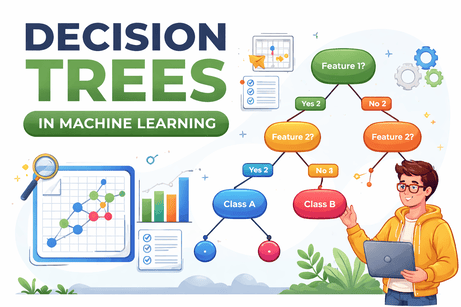
Decision Trees are supervised machine learning algorithms used for both classification and regression. In scikit-learn, the main classes are DecisionTreeClassifier and DecisionTreeRegressor. A tree works by recursively splitting the data into smaller regions using feature-based rules until it reaches a prediction at a leaf node.
1) What a Decision Tree does
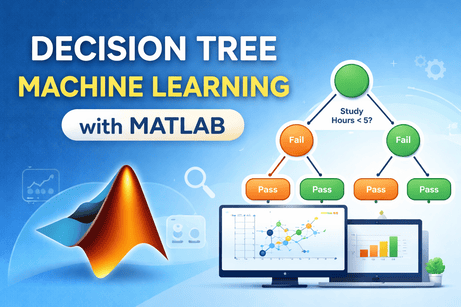
A Decision Tree learns a sequence of if-then rules from data.
Example:
- if
age < 30, go left - if
salary > 5000, go right - if
experience < 2, go left again
At the end of the path, the model reaches a leaf and makes a prediction.
So a tree is built from:
- a root node: the first split
- internal nodes: decision rules
- branches: the outcomes of rules
- leaf nodes: final predictions
This makes Decision Trees one of the easiest machine learning models to understand visually. Scikit-learn also provides plot_tree to visualize a fitted tree.
2) Why Decision Trees are useful
Decision Trees are popular because they are:
- easy to interpret
- able to model nonlinear relationships
- usable for classification and regression
- able to handle numerical and, after preprocessing, categorical-style encoded features
They are also a foundation for more advanced ensemble models such as Random Forests and Gradient Boosting. Scikit-learn describes Random Forests as ensembles of decision trees built on subsamples to improve predictive accuracy and control overfitting.
3) How a Decision Tree chooses splits
At each node, the tree searches for the split that best separates the data.
For classification, DecisionTreeClassifier supports criteria such as:
ginientropylog_loss
For regression, DecisionTreeRegressor supports criteria such as:
squared_errorfriedman_mseabsolute_errorpoisson
Classification intuition
A good split is one that makes the child nodes more “pure”.
Example:
- one branch contains mostly class A
- the other branch contains mostly class B
That is better than a split where both branches remain mixed.
Regression intuition
A good split reduces prediction error inside each child node.
Example:
- one branch contains mostly low target values
- the other contains mostly high target values
4) Decision Tree for classification
In classification, each leaf predicts a class. Scikit-learn’s tree guide notes that DecisionTreeClassifier supports binary and multiclass classification, and it can also output class probabilities with predict_proba, where the probability is based on the fraction of training samples of each class in the leaf.
Example
Suppose the tree is predicting whether a student passes:
- if hours studied > 4
- and attendance > 80%
- then predict Pass
Otherwise:
- predict Fail
This is why trees are very interpretable.
5) Decision Tree for regression
In regression, each leaf predicts a number.
Example:
- if house size > 120 m² and neighborhood score > 7
- then predict price = 1,500,000
Otherwise:
- predict another value
Unlike linear regression, a decision tree regressor does not fit one global equation. It splits the feature space into regions and predicts a value in each region. Scikit-learn’s regression example shows that tree regression can approximate a nonlinear sine curve, but can overfit noise when max_depth is too high.
6) Why Decision Trees do not need feature scaling
Unlike SVM and KNN, Decision Trees do not depend on geometric distance. They split on thresholds like:
feature <= valuefeature > value
Because of that, feature scaling is usually not necessary for tree models. This follows from how scikit-learn decision trees operate: they choose threshold-based splits feature by feature rather than optimizing a distance-based objective.
So this is one major practical advantage of trees.
Part I — First Classification Example
7) Install required libraries
pip install numpy pandas matplotlib scikit-learn8) A simple Decision Tree classification example
We will use the Breast Cancer dataset from scikit-learn.
import numpy as np
import pandas as pd

from sklearn.datasets import load_breast_cancer
from sklearn.model_selection import train_test_split
from sklearn.tree import DecisionTreeClassifier
from sklearn.metrics import accuracy_score, classification_report, confusion_matrix

# Load dataset
data = load_breast_cancer()
X = data.data
y = data.target

# Split
X_train, X_test, y_train, y_test = train_test_split(
    X, y, test_size=0.2, random_state=42, stratify=y
)

# Build model
model = DecisionTreeClassifier(random_state=42)

# Train
model.fit(X_train, y_train)

# Predict
y_pred = model.predict(X_test)

# Evaluate
print("Accuracy:", accuracy_score(y_test, y_pred))
print("\nConfusion Matrix:\n", confusion_matrix(y_test, y_pred))
print("\nClassification Report:\n", classification_report(y_test, y_pred))
What this code does
- loads the dataset
- splits it into train and test sets
- trains a Decision Tree classifier
- predicts on the test set
- evaluates the model
DecisionTreeClassifier uses criterion, splitter, max_depth, and other parameters to control how the tree is built.
9) Predicting class probabilities
A Decision Tree can also estimate probabilities.
proba = model.predict_proba(X_test[:5])
print(proba)
This returns the class probabilities for the first five samples. In scikit-learn, these probabilities are based on the class proportions in the leaf reached by each sample.
Part II — Visualizing a Tree
10) Plot the tree
Scikit-learn provides plot_tree to visualize a fitted decision tree. It can show node labels, class names, feature names, impurity, and sample counts.
import matplotlib.pyplot as plt
from sklearn.tree import plot_tree

plt.figure(figsize=(20, 10))
plot_tree(
    model,
    filled=True,
    feature_names=data.feature_names,
    class_names=data.target_names,
    rounded=True,
    fontsize=8
)
plt.show()
What you will see
Each node typically shows:
- the feature used for the split
- the threshold
- impurity
- number of samples
- class distribution
- predicted class
This is one of the best parts of using Decision Trees: you can inspect the learned logic directly.
11) Limit tree depth for readability
Very large trees become hard to read.
plt.figure(figsize=(18, 8))
plot_tree(
    model,
    max_depth=3,
    filled=True,
    feature_names=data.feature_names,
    class_names=data.target_names,
    rounded=True,
    fontsize=9
)
plt.show()
The plot_tree function supports a max_depth argument, which is useful for visualization even if the underlying model is deeper.
Part III — Important Parameters
12) Key parameters for DecisionTreeClassifier
From the scikit-learn API, important parameters include:
criterionsplittermax_depthmin_samples_splitmin_samples_leafmax_featuresrandom_stateccp_alpha
criterion
Measures split quality.
Common choices:
ginientropylog_loss
max_depth
Maximum depth of the tree.
- small depth → simpler model
- large depth → more complex model
min_samples_split
Minimum number of samples required to split a node.
min_samples_leaf
Minimum number of samples required in a leaf.
splitter
Can be:
"best""random"
ccp_alpha
Controls minimal cost-complexity pruning. Scikit-learn added pruning controlled by ccp_alpha for tree estimators; increasing it prunes the tree more aggressively.
13) Why trees overfit easily
Decision Trees are flexible. That is useful, but it also means they can memorize training data.
Signs of overfitting:
- very high training accuracy
- much lower test accuracy
- extremely deep tree
- many leaves with very few samples
Scikit-learn’s tree regression example explicitly notes that high max_depth can make the model learn the noise and overfit.
14) Common ways to control overfitting
You can regularize a tree by limiting its growth:
max_depthmin_samples_splitmin_samples_leafmax_leaf_nodesccp_alpha
Example:
model = DecisionTreeClassifier(
    max_depth=4,
    min_samples_split=10,
    min_samples_leaf=5,
    random_state=42
)
This usually generalizes better than an unconstrained tree.
Part IV — Tuning a Decision Tree
15) Tune with GridSearchCV
GridSearchCV is the standard scikit-learn tool for exhaustive hyperparameter search with cross-validation.
from sklearn.model_selection import GridSearchCV
from sklearn.tree import DecisionTreeClassifier

param_grid = {
    "criterion": ["gini", "entropy", "log_loss"],
    "max_depth": [3, 5, 7, 10, None],
    "min_samples_split": [2, 5, 10, 20],
    "min_samples_leaf": [1, 2, 4, 8]
}

grid = GridSearchCV(
    estimator=DecisionTreeClassifier(random_state=42),
    param_grid=param_grid,
    cv=5,
    scoring="accuracy",
    n_jobs=-1
)

grid.fit(X_train, y_train)

print("Best Parameters:", grid.best_params_)
print("Best CV Score:", grid.best_score_)

best_model = grid.best_estimator_
y_pred = best_model.predict(X_test)
print("Test Accuracy:", accuracy_score(y_test, y_pred))
Why this is useful
Instead of guessing the best depth or leaf size, you let cross-validation choose a stronger configuration.
16) Pruning with ccp_alpha
Cost-complexity pruning is one of the most important practical tools for trees in scikit-learn. The pruning control parameter is ccp_alpha. Larger values prune more nodes.
Example:
pruned_model = DecisionTreeClassifier(
    random_state=42,
    ccp_alpha=0.01
)

pruned_model.fit(X_train, y_train)
y_pred = pruned_model.predict(X_test)

print("Pruned Accuracy:", accuracy_score(y_test, y_pred))
Intuition
Pruning removes branches that add complexity but do not improve generalization enough.
Part V — Visual Example on 2D Data
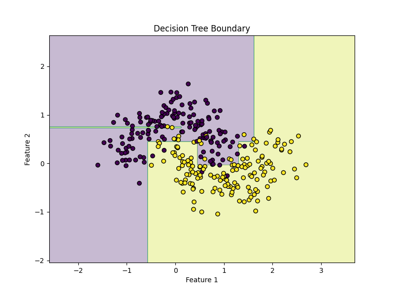
17) Decision Tree on a synthetic dataset
We will use make_moons to see a nonlinear decision boundary.
import matplotlib.pyplot as plt
import numpy as np

from sklearn.datasets import make_moons
from sklearn.model_selection import train_test_split
from sklearn.tree import DecisionTreeClassifier

# Create nonlinear dataset
X, y = make_moons(n_samples=300, noise=0.25, random_state=42)

X_train, X_test, y_train, y_test = train_test_split(
    X, y, test_size=0.2, random_state=42
)

model = DecisionTreeClassifier(max_depth=5, random_state=42)
model.fit(X_train, y_train)

print("Accuracy:", model.score(X_test, y_test))
Plot decision boundary
def plot_decision_boundary(model, X, y):
    x_min, x_max = X[:, 0].min() - 1, X[:, 0].max() + 1
    y_min, y_max = X[:, 1].min() - 1, X[:, 1].max() + 1

    xx, yy = np.meshgrid(
        np.linspace(x_min, x_max, 400),
        np.linspace(y_min, y_max, 400)
    )

    Z = model.predict(np.c_[xx.ravel(), yy.ravel()])
    Z = Z.reshape(xx.shape)

    plt.figure(figsize=(8, 6))
    plt.contourf(xx, yy, Z, alpha=0.3)
    plt.scatter(X[:, 0], X[:, 1], c=y, edgecolors="k")
    plt.title("Decision Tree Boundary")
    plt.xlabel("Feature 1")
    plt.ylabel("Feature 2")
    plt.show()

plot_decision_boundary(model, X, y)
What you will notice
Decision Tree boundaries are made of axis-aligned splits, so they often look like rectangular step-like regions rather than smooth curves.
18) Effect of depth
for depth in [1, 3, 5, 10, None]:
    model = DecisionTreeClassifier(max_depth=depth, random_state=42)
    model.fit(X_train, y_train)
    print(f"max_depth={depth}, accuracy={model.score(X_test, y_test):.4f}")
Interpretation
- shallow tree → simpler boundary
- deeper tree → more complex boundary
- very deep tree → risk of overfitting
This matches scikit-learn’s warning from the tree regression example that too much depth can fit noise rather than signal.
Part VI — Decision Tree Regression
19) Example with DecisionTreeRegressor
Now let us use a Decision Tree for regression.
import numpy as np
import matplotlib.pyplot as plt

from sklearn.tree import DecisionTreeRegressor
from sklearn.model_selection import train_test_split
from sklearn.metrics import mean_squared_error, r2_score

# Synthetic data
rng = np.random.RandomState(42)
X = np.sort(5 * rng.rand(200, 1), axis=0)
y = np.sin(X).ravel()

# Add noise
y[::5] += 0.5 - rng.rand(40)

X_train, X_test, y_train, y_test = train_test_split(
    X, y, test_size=0.2, random_state=42
)

model = DecisionTreeRegressor(max_depth=4, random_state=42)

model.fit(X_train, y_train)
y_pred = model.predict(X_test)

print("MSE:", mean_squared_error(y_test, y_pred))
print("R²:", r2_score(y_test, y_pred))
Plot predictions
X_plot = np.linspace(X.min(), X.max(), 500).reshape(-1, 1)
y_plot = model.predict(X_plot)

plt.figure(figsize=(8, 6))
plt.scatter(X, y, label="Data")
plt.plot(X_plot, y_plot, linewidth=2, label="Tree prediction")
plt.xlabel("X")
plt.ylabel("y")
plt.title("Decision Tree Regression")
plt.legend()
plt.show()
Scikit-learn’s official tree regression example uses a similar sine-style dataset and shows how tree depth changes the fit quality.
20) Important regression parameters
DecisionTreeRegressor shares many structure-control parameters with the classifier version, including:
max_depthmin_samples_splitmin_samples_leafmax_featuresccp_alpha
Its split criterion options include:
squared_errorfriedman_mseabsolute_errorpoisson
Example:
model = DecisionTreeRegressor(
    criterion="squared_error",
    max_depth=5,
    min_samples_leaf=4,
    random_state=42
)
Part VII — A Full Real Workflow
21) End-to-end classification workflow
Step 1: Load data
import pandas as pd

df = pd.read_csv("your_data.csv")
Step 2: Separate features and target
X = df.drop("target", axis=1)
y = df["target"]
Step 3: Split data
from sklearn.model_selection import train_test_split

X_train, X_test, y_train, y_test = train_test_split(
    X, y, test_size=0.2, random_state=42, stratify=y
)
Step 4: Build model
from sklearn.tree import DecisionTreeClassifier

model = DecisionTreeClassifier(random_state=42)
Step 5: Tune parameters
from sklearn.model_selection import GridSearchCV

param_grid = {
    "criterion": ["gini", "entropy", "log_loss"],
    "max_depth": [3, 5, 7, 10, None],
    "min_samples_split": [2, 5, 10],
    "min_samples_leaf": [1, 2, 4]
}

grid = GridSearchCV(
    model,
    param_grid=param_grid,
    cv=5,
    scoring="accuracy",
    n_jobs=-1
)

grid.fit(X_train, y_train)
Step 6: Evaluate
from sklearn.metrics import classification_report, confusion_matrix, accuracy_score

best_model = grid.best_estimator_
y_pred = best_model.predict(X_test)

print("Best Params:", grid.best_params_)
print("Accuracy:", accuracy_score(y_test, y_pred))
print(confusion_matrix(y_test, y_pred))
print(classification_report(y_test, y_pred))
Step 7: Predict on new samples
new_samples = X_test.iloc[:5]
predictions = best_model.predict(new_samples)
print(predictions)
Part VIII — Understanding Tree Structure
22) Inspecting the fitted tree
Scikit-learn’s example on understanding tree structure explains that a fitted tree has a tree_ attribute containing low-level information like node_count and max_depth.
Example:
print("Node count:", model.tree_.node_count)
print("Max depth:", model.tree_.max_depth)
This can be useful for diagnosing model complexity.
23) Feature importance
Decision Trees in scikit-learn expose feature_importances_, which summarizes the relative importance of each feature in the fitted tree.
import pandas as pd

importance = pd.Series(model.feature_importances_, index=data.feature_names)
print(importance.sort_values(ascending=False))
This is often useful, but interpret it carefully: tree-based feature importance can be biased in some situations, so it is best used as an exploratory signal rather than absolute truth. This caution is an inference based on how impurity-based splitting works in trees.
Part IX — How to Read the Results
24) Classification metrics
For classification, common metrics are:
- accuracy
- precision
- recall
- F1-score
- confusion matrix
from sklearn.metrics import confusion_matrix, classification_report

print(confusion_matrix(y_test, y_pred))
print(classification_report(y_test, y_pred))
Decision trees support multiclass classification as well as binary classification, so these metrics work naturally in many common settings.
25) Regression metrics
For regression, common metrics are:
- MAE
- MSE
- RMSE
- R²
from sklearn.metrics import mean_absolute_error, mean_squared_error, r2_score
import numpy as np

mae = mean_absolute_error(y_test, y_pred)
mse = mean_squared_error(y_test, y_pred)
rmse = np.sqrt(mse)
r2 = r2_score(y_test, y_pred)

print("MAE:", mae)
print("MSE:", mse)
print("RMSE:", rmse)
print("R²:", r2)
Part X — Strengths and Weaknesses
26) Strengths of Decision Trees
Decision Trees are strong because they are:
- interpretable
- able to model nonlinear relationships
- usable without feature scaling
- capable of handling classification and regression
They also form the basis of important ensemble methods such as Random Forests and Gradient Boosting.
27) Weaknesses of Decision Trees
Their main weaknesses are:
- they overfit easily
- they can be unstable to small data changes
- they often produce axis-aligned, blocky boundaries
- a single tree may have lower predictive power than ensembles
This is one reason scikit-learn highlights ensemble tree methods alongside single trees.
Part XI — Common Mistakes
28) Letting the tree grow without limits
Bad:
model = DecisionTreeClassifier(random_state=42)This can work, but it may overfit badly.
Better:
model = DecisionTreeClassifier(
    max_depth=5,
    min_samples_leaf=4,
    random_state=42
)
29) Ignoring pruning
Many users tune depth but forget ccp_alpha. Minimal cost-complexity pruning is built into scikit-learn trees and can be very effective for reducing overfitting.
30) Interpreting feature importance too literally
Feature importance in a single tree can be useful, but it is not the same thing as causal importance. Treat it as a model-based summary, not proof of real-world causation.
Part XII — Practical Advice
31) When should you use a Decision Tree?
Use a Decision Tree when:
- interpretability matters
- you want clear if-then rules
- you want a quick baseline
- the relationship may be nonlinear
- you do not want to worry about scaling
32) When should you avoid a single tree?
Be careful with a single tree when:
- maximum predictive accuracy is your top goal
- the dataset is noisy
- the model overfits easily
- you need more stability
In those cases, ensemble models like Random Forests or Gradient Boosting are often stronger follow-up options.
33) A good default starting point
For classification:
DecisionTreeClassifier(
    criterion="gini",
    max_depth=5,
    min_samples_leaf=4,
    random_state=42
)
For regression:
DecisionTreeRegressor(
    criterion="squared_error",
    max_depth=5,
    min_samples_leaf=4,
    random_state=42
)
These are not universal best settings, but they are sensible starting points to reduce overfitting compared with a completely unconstrained tree. The available criteria and structure-control parameters are documented in the scikit-learn API.
Part XIII — Mini Project Example
34) Predicting iris species with a Decision Tree
from sklearn.datasets import load_iris
from sklearn.model_selection import train_test_split, GridSearchCV
from sklearn.tree import DecisionTreeClassifier
from sklearn.metrics import classification_report, confusion_matrix, accuracy_score

# Load
data = load_iris()
X, y = data.data, data.target

# Split
X_train, X_test, y_train, y_test = train_test_split(
    X, y, test_size=0.2, stratify=y, random_state=42
)

# Model
model = DecisionTreeClassifier(random_state=42)

# Search space
param_grid = {
    "criterion": ["gini", "entropy", "log_loss"],
    "max_depth": [2, 3, 4, 5, None],
    "min_samples_split": [2, 5, 10],
    "min_samples_leaf": [1, 2, 4]
}

# Grid search
grid = GridSearchCV(
    model,
    param_grid=param_grid,
    cv=5,
    scoring="accuracy",
    n_jobs=-1
)

grid.fit(X_train, y_train)

# Evaluate
best_model = grid.best_estimator_
y_pred = best_model.predict(X_test)

print("Best Parameters:", grid.best_params_)
print("Accuracy:", accuracy_score(y_test, y_pred))
print("\nConfusion Matrix:\n", confusion_matrix(y_test, y_pred))
print("\nClassification Report:\n", classification_report(y_test, y_pred))
Why this mini-project is good
- uses a train/test split
- tunes the most important structural parameters
- evaluates on held-out data
- stays easy to interpret
Part XIV — Summary
35) What you should remember
Decision Trees are one of the easiest machine learning models to understand.
The core idea is:
- split the data into smaller regions
- use if-then rules
- predict from the leaf reached by each sample
For classification, the tree predicts a class or class probabilities. For regression, it predicts a numeric value. Scikit-learn supports both through DecisionTreeClassifier and DecisionTreeRegressor.
The most important practical rules are:
- feature scaling is usually not needed
- control complexity with
max_depth,min_samples_leaf, andmin_samples_split - consider
ccp_alphafor pruning - use cross-validation
- visualize the tree when interpretability matters
These recommendations align with the current scikit-learn documentation for decision trees and tree visualization.
36) Final ready-to-use template
from sklearn.model_selection import train_test_split, GridSearchCV
from sklearn.tree import DecisionTreeClassifier
from sklearn.metrics import classification_report

# X, y = your data

X_train, X_test, y_train, y_test = train_test_split(
    X, y, test_size=0.2, random_state=42
)

model = DecisionTreeClassifier(random_state=42)

param_grid = {
    "criterion": ["gini", "entropy", "log_loss"],
    "max_depth": [3, 5, 7, None],
    "min_samples_split": [2, 5, 10],
    "min_samples_leaf": [1, 2, 4]
}

grid = GridSearchCV(
    model,
    param_grid=param_grid,
    cv=5,
    scoring="accuracy",
    n_jobs=-1
)

grid.fit(X_train, y_train)

print("Best params:", grid.best_params_)
print("Test score:", grid.best_estimator_.score(X_test, y_test))

y_pred = grid.best_estimator_.predict(X_test)
print(classification_report(y_test, y_pred))
37) Practice exercises
Exercise 1
Train a DecisionTreeClassifier on the Iris dataset and report accuracy.
Exercise 2
Train a Decision Tree on make_moons and visualize the decision boundary.
Exercise 3
Tune max_depth, min_samples_split, and min_samples_leaf using GridSearchCV.
Exercise 4
Compare an unconstrained tree with a pruned or depth-limited tree.
Exercise 5
Train a DecisionTreeRegressor on a nonlinear synthetic regression dataset.
Final summary
What each exercise teaches
- Exercise 1: basic Decision Tree classification
- Exercise 2: nonlinear classification and decision-boundary visualization
- Exercise 3: hyperparameter tuning
- Exercise 4: comparing a full tree with a simpler or pruned tree
- Exercise 5: nonlinear regression with a Decision Tree









💬 Comments
No comments yet. Be the first to comment!
Login to comment.