0) Introduction
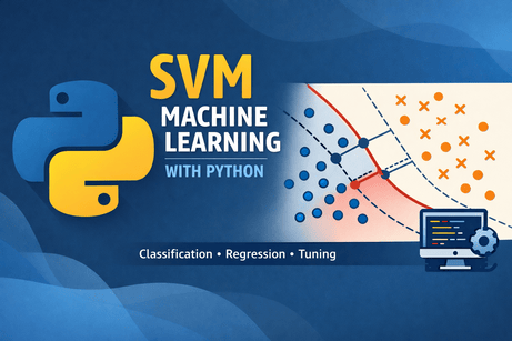
Support Vector Machines, or SVMs, are supervised learning algorithms used for classification and regression. In scikit-learn, the main classes are SVC and LinearSVC for classification, and SVR and LinearSVR for regression. The official scikit-learn guide also notes that SVMs are effective in high-dimensional spaces, can still work well when the number of features is larger than the number of samples, and use only a subset of the training points in the decision function, called support vectors.
1) What an SVM does
Imagine you have two classes of points, for example:
- class 0: red points
- class 1: blue points
An SVM tries to find a boundary that separates them. But it does not choose just any boundary. It chooses the one with the largest margin, meaning the widest possible gap between the classes.
That is the central idea:
- decision boundary: the line, plane, or hypersurface separating classes
- margin: the distance between the boundary and the nearest training points
- support vectors: the points closest to the boundary; they “support” and define the classifier
In practice, this often gives good generalization on unseen data.
2) Why SVM is powerful
SVM is useful when:
- the dataset is small or medium-sized
- the classes are separable or almost separable
- there are many features
- you want a strong baseline model
Scikit-learn also warns that SVC is based on libsvm and that fit time scales at least quadratically with the number of samples, so it may become impractical beyond tens of thousands of samples. For larger datasets, the docs recommend considering LinearSVC or SGDClassifier, possibly with kernel approximation techniques.
3) Linear SVM intuition
Suppose your data has only 2 features:
- feature 1 = exam score
- feature 2 = hours studied
A linear SVM tries to draw a straight line that separates “pass” from “fail”.
If several lines can separate the classes, the SVM picks the one with the largest margin.
Hard margin vs soft margin
Hard margin
Used when the data is perfectly separable.
The model insists on zero classification error.
Soft margin
Used when the data is noisy.
The model allows some mistakes but still tries to maximize the margin.
This is controlled by the parameter C.
- small
C: wider margin, more tolerance for mistakes, stronger regularization - large
C: fewer mistakes on training data, narrower margin, weaker regularization
4) Nonlinear SVM and the kernel trick
Real data is often not linearly separable.
Example:
- points of class A are in the center
- points of class B surround them in a circle
A straight line cannot separate them.
SVM solves this using kernels. A kernel lets the algorithm act as if it mapped data into a higher-dimensional space without explicitly computing that mapping. Scikit-learn’s SVC supports kernels such as linear, polynomial, RBF, and sigmoid.
Common kernels:
- linear
- poly
- rbf (most popular nonlinear choice)
- sigmoid
RBF kernel
The RBF kernel is often the default and a very strong general-purpose choice.
Important parameter:
gamma
Interpretation:
- small
gamma: smoother, broader influence of each point - large
gamma: more localized influence, more complex boundary
So with RBF SVM, the two most important tuning parameters are usually:
Cgamma
5) SVM for regression
SVM is not only for classification.
For regression, scikit-learn provides SVR and LinearSVR. The regression version tries to fit a function while allowing an error tolerance band, controlled by epsilon, around the prediction. SVR uses libsvm and nonlinear kernels if desired, while LinearSVR is designed to scale better for larger datasets.
Main regression parameters:
C: regularizationepsilon: width of the no-penalty tubekernel: for nonlinear regressiongamma: for RBF/poly/sigmoid kernels
6) Why feature scaling matters a lot
SVM is very sensitive to feature scales.
Example:
- age ranges from 18 to 60
- salary ranges from 1,000 to 100,000
Without scaling, salary may dominate the geometry of the model.
That is why standardization is strongly recommended. StandardScaler standardizes features by removing the mean and scaling to unit variance. In scikit-learn, a Pipeline is the recommended way to chain preprocessing and the final estimator so training and prediction use the exact same transformations.
Part I — First Classification Example
7) Install required libraries
pip install numpy pandas matplotlib scikit-learn8) A simple linear SVM classification example
We will use the Breast Cancer dataset from scikit-learn.
import numpy as np
import pandas as pd

from sklearn.datasets import load_breast_cancer
from sklearn.model_selection import train_test_split
from sklearn.pipeline import Pipeline
from sklearn.preprocessing import StandardScaler
from sklearn.svm import SVC
from sklearn.metrics import accuracy_score, classification_report, confusion_matrix

# Load dataset
data = load_breast_cancer()
X = data.data
y = data.target

# Split
X_train, X_test, y_train, y_test = train_test_split(
    X, y, test_size=0.2, random_state=42, stratify=y
)

# Pipeline: scaling + linear SVM
model = Pipeline([
    ("scaler", StandardScaler()),
    ("svm", SVC(kernel="linear", C=1.0))
])

# Train
model.fit(X_train, y_train)

# Predict
y_pred = model.predict(X_test)

# Evaluate
print("Accuracy:", accuracy_score(y_test, y_pred))
print("\nConfusion Matrix:\n", confusion_matrix(y_test, y_pred))
print("\nClassification Report:\n", classification_report(y_test, y_pred))
What this code does
- loads the dataset
- splits it into train and test sets
- scales the features
- trains a linear SVM classifier
- evaluates the model
Why use a pipeline
Because Pipeline applies preprocessing and prediction in sequence, it prevents mistakes such as fitting the scaler outside the cross-validation loop or forgetting to scale new data before predicting. That is exactly what the scikit-learn pipeline API is for.
9) A nonlinear SVM with RBF kernel
Now let us switch to a nonlinear model.
from sklearn.pipeline import Pipeline
from sklearn.preprocessing import StandardScaler
from sklearn.svm import SVC

rbf_model = Pipeline([
    ("scaler", StandardScaler()),
    ("svm", SVC(kernel="rbf", C=1.0, gamma="scale"))
])

rbf_model.fit(X_train, y_train)
y_pred_rbf = rbf_model.predict(X_test)

print("RBF Accuracy:", accuracy_score(y_test, y_pred_rbf))
print("\nConfusion Matrix:\n", confusion_matrix(y_test, y_pred_rbf))
print("\nClassification Report:\n", classification_report(y_test, y_pred_rbf))
Why gamma="scale"?
That is the modern scikit-learn default for SVC, and it is usually a sensible starting point.
Part II — Visual Example on 2D Data
10) SVM on a synthetic dataset
This is a good way to understand the decision boundary.
import matplotlib.pyplot as plt

from sklearn.datasets import make_moons
from sklearn.model_selection import train_test_split
from sklearn.pipeline import Pipeline
from sklearn.preprocessing import StandardScaler
from sklearn.svm import SVC

# Create nonlinear dataset
X, y = make_moons(n_samples=300, noise=0.2, random_state=42)

X_train, X_test, y_train, y_test = train_test_split(
    X, y, test_size=0.2, random_state=42
)

model = Pipeline([
    ("scaler", StandardScaler()),
    ("svm", SVC(kernel="rbf", C=1.0, gamma="scale"))
])

model.fit(X_train, y_train)

print("Accuracy:", model.score(X_test, y_test))
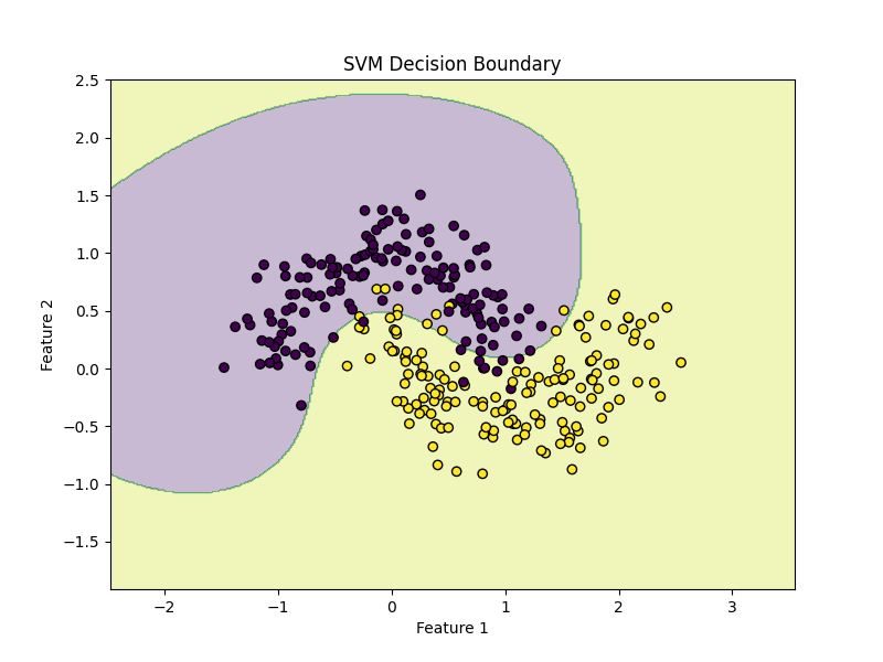
Plot the decision boundary
import numpy as np
import matplotlib.pyplot as plt

def plot_decision_boundary(model, X, y):
    x_min, x_max = X[:, 0].min() - 1, X[:, 0].max() + 1
    y_min, y_max = X[:, 1].min() - 1, X[:, 1].max() + 1

    xx, yy = np.meshgrid(
        np.linspace(x_min, x_max, 400),
        np.linspace(y_min, y_max, 400)
    )

    Z = model.predict(np.c_[xx.ravel(), yy.ravel()])
    Z = Z.reshape(xx.shape)

    plt.figure(figsize=(8, 6))
    plt.contourf(xx, yy, Z, alpha=0.3)
    plt.scatter(X[:, 0], X[:, 1], c=y, edgecolors="k")
    plt.title("SVM Decision Boundary")
    plt.xlabel("Feature 1")
    plt.ylabel("Feature 2")
    plt.show()

plot_decision_boundary(model, X, y)
This plot helps you see how the RBF kernel creates a curved boundary.
Part III — Hyperparameter Tuning
11) The most important SVM parameters
For classification with SVC
kernel: linear, rbf, poly, sigmoidC: regularization strengthgamma: kernel coefficient for nonlinear kernelsdegree: for polynomial kernel
For regression with SVR
Cepsilongammakernel
12) Tune SVM with GridSearchCV
Scikit-learn’s GridSearchCV performs an exhaustive search over parameter combinations with cross-validation. The documentation recommends it for hyperparameter tuning when you want a systematic search over a specified grid.
from sklearn.model_selection import GridSearchCV

pipeline = Pipeline([
    ("scaler", StandardScaler()),
    ("svm", SVC())
])

param_grid = {
    "svm__kernel": ["linear", "rbf"],
    "svm__C": [0.1, 1, 10, 100],
    "svm__gamma": ["scale", 0.01, 0.1, 1]
}

grid = GridSearchCV(
    estimator=pipeline,
    param_grid=param_grid,
    cv=5,
    scoring="accuracy",
    n_jobs=-1
)

grid.fit(X_train, y_train)

print("Best Parameters:", grid.best_params_)
print("Best CV Score:", grid.best_score_)

best_model = grid.best_estimator_
test_score = best_model.score(X_test, y_test)
print("Test Accuracy:", test_score)
Important note
If kernel="linear", gamma is irrelevant.
Still, it is common in simple tutorials to keep one shared grid. In a production project, you may separate the parameter grid by kernel type.
Example:
param_grid = [
    {
        "svm__kernel": ["linear"],
        "svm__C": [0.1, 1, 10, 100]
    },
    {
        "svm__kernel": ["rbf"],
        "svm__C": [0.1, 1, 10, 100],
        "svm__gamma": ["scale", 0.01, 0.1, 1]
    }
]
This is cleaner.
13) Faster search with RandomizedSearchCV
If the search space is large, RandomizedSearchCV can be more efficient because it samples a fixed number of parameter settings rather than testing all combinations. Scikit-learn documents it as the sampling-based alternative to GridSearchCV.
from sklearn.model_selection import RandomizedSearchCV
from scipy.stats import loguniform

pipeline = Pipeline([
    ("scaler", StandardScaler()),
    ("svm", SVC(kernel="rbf"))
])

param_dist = {
    "svm__C": loguniform(1e-2, 1e2),
    "svm__gamma": loguniform(1e-3, 1e1)
}

random_search = RandomizedSearchCV(
    pipeline,
    param_distributions=param_dist,
    n_iter=20,
    cv=5,
    scoring="accuracy",
    n_jobs=-1,
    random_state=42
)

random_search.fit(X_train, y_train)

print("Best Parameters:", random_search.best_params_)
print("Best CV Score:", random_search.best_score_)
print("Test Accuracy:", random_search.best_estimator_.score(X_test, y_test))
Part IV — Understanding SVC vs LinearSVC
14) What is the difference?
Scikit-learn documents that:
SVC(kernel="linear")uses libsvmLinearSVCuses liblinearLinearSVCgenerally scales better to large datasets- there are differences in optimization details and defaults between them
Rule of thumb
Use:
SVC(kernel="linear")for small/medium datasets when you want the classic SVM formulationLinearSVCfor larger linear problemsSVC(kernel="rbf")when the boundary is nonlinear
Example with LinearSVC
from sklearn.svm import LinearSVC

linear_svc_model = Pipeline([
    ("scaler", StandardScaler()),
    ("svm", LinearSVC(C=1.0, max_iter=10000))
])

linear_svc_model.fit(X_train, y_train)
y_pred = linear_svc_model.predict(X_test)

print("Accuracy:", accuracy_score(y_test, y_pred))
print("\nClassification Report:\n", classification_report(y_test, y_pred))
Part V — SVM Regression with Python
15) Example with SVR
Let us create a synthetic regression problem.
import numpy as np
import matplotlib.pyplot as plt

from sklearn.svm import SVR
from sklearn.pipeline import Pipeline
from sklearn.preprocessing import StandardScaler
from sklearn.model_selection import train_test_split
from sklearn.metrics import mean_squared_error, r2_score

# Synthetic data
rng = np.random.RandomState(42)
X = np.sort(5 * rng.rand(200, 1), axis=0)
y = np.sin(X).ravel()

# Add noise
y[::5] += 0.5 - rng.rand(40)

X_train, X_test, y_train, y_test = train_test_split(
    X, y, test_size=0.2, random_state=42
)

model = Pipeline([
    ("scaler", StandardScaler()),
    ("svr", SVR(kernel="rbf", C=10, epsilon=0.1, gamma="scale"))
])

model.fit(X_train, y_train)
y_pred = model.predict(X_test)

print("MSE:", mean_squared_error(y_test, y_pred))
print("R²:", r2_score(y_test, y_pred))

Plot predictions

X_plot = np.linspace(X.min(), X.max(), 500).reshape(-1, 1)
y_plot = model.predict(X_plot)

plt.figure(figsize=(8, 6))
plt.scatter(X, y, label="Data")
plt.plot(X_plot, y_plot, linewidth=2, label="SVR prediction")
plt.xlabel("X")
plt.ylabel("y")
plt.title("Support Vector Regression")
plt.legend()
plt.show()
16) Example with LinearSVR
If the relationship is approximately linear and the dataset is large, LinearSVR can be faster. Scikit-learn distinguishes it from SVR in the same way LinearSVC differs from SVC: better scalability for linear settings.
from sklearn.svm import LinearSVR

linear_svr_model = Pipeline([
    ("scaler", StandardScaler()),
    ("svr", LinearSVR(C=1.0, epsilon=0.1, max_iter=10000))
])

linear_svr_model.fit(X_train, y_train)
y_pred = linear_svr_model.predict(X_test)

print("MSE:", mean_squared_error(y_test, y_pred))
print("R²:", r2_score(y_test, y_pred))
Part VI — A Full Real Workflow
17) End-to-end classification workflow
This is the workflow you should use in real projects.
Step 1: Load data
import pandas as pd

df = pd.read_csv("your_data.csv")
Step 2: Separate features and target
X = df.drop("target", axis=1)
y = df["target"]
Step 3: Split data
from sklearn.model_selection import train_test_split

X_train, X_test, y_train, y_test = train_test_split(
    X, y, test_size=0.2, random_state=42, stratify=y
)
Step 4: Build pipeline
from sklearn.pipeline import Pipeline
from sklearn.preprocessing import StandardScaler
from sklearn.svm import SVC

pipeline = Pipeline([
    ("scaler", StandardScaler()),
    ("svm", SVC())
])
Step 5: Tune parameters
from sklearn.model_selection import GridSearchCV

param_grid = [
    {
        "svm__kernel": ["linear"],
        "svm__C": [0.1, 1, 10]
    },
    {
        "svm__kernel": ["rbf"],
        "svm__C": [0.1, 1, 10],
        "svm__gamma": ["scale", 0.01, 0.1, 1]
    }
]

grid = GridSearchCV(
    pipeline,
    param_grid=param_grid,
    cv=5,
    scoring="accuracy",
    n_jobs=-1
)

grid.fit(X_train, y_train)
Step 6: Evaluate
from sklearn.metrics import classification_report, confusion_matrix, accuracy_score

best_model = grid.best_estimator_
y_pred = best_model.predict(X_test)

print("Best Params:", grid.best_params_)
print("Accuracy:", accuracy_score(y_test, y_pred))
print(confusion_matrix(y_test, y_pred))
print(classification_report(y_test, y_pred))
Step 7: Predict on new samples
new_samples = X_test.iloc[:5]
predictions = best_model.predict(new_samples)
print(predictions)
Part VII — SVM with Text Data
18) SVM is excellent for text classification
SVM, especially linear SVM, is a classic strong method for text classification because text data often has very high dimensional sparse features. Scikit-learn’s text tutorial shows the standard pattern of turning text into feature vectors and then training a classifier in a pipeline.
Example:
from sklearn.pipeline import Pipeline
from sklearn.feature_extraction.text import TfidfVectorizer
from sklearn.svm import LinearSVC
from sklearn.model_selection import train_test_split
from sklearn.metrics import classification_report

texts = [
    "I love this product",
    "This is amazing",
    "Very bad quality",
    "I hate it",
    "Excellent and wonderful",
    "Terrible experience"
]

labels = [1, 1, 0, 0, 1, 0]  # 1 = positive, 0 = negative

X_train, X_test, y_train, y_test = train_test_split(
    texts, labels, test_size=0.3, random_state=42
)

text_model = Pipeline([
    ("tfidf", TfidfVectorizer()),
    ("clf", LinearSVC())
])

text_model.fit(X_train, y_train)
y_pred = text_model.predict(X_test)

print(classification_report(y_test, y_pred))
This is a simple sentiment classification example.
Part VIII — How to Read the Results
19) Classification metrics
For classification, common metrics are:
- accuracy
- precision
- recall
- F1-score
- confusion matrix
Use accuracy when classes are balanced.
If classes are imbalanced, pay more attention to precision, recall, and F1.
Example:
from sklearn.metrics import confusion_matrix, classification_report

print(confusion_matrix(y_test, y_pred))
print(classification_report(y_test, y_pred))
20) Regression metrics
For regression, common metrics are:
- MAE
- MSE
- RMSE
- R²
Example:
from sklearn.metrics import mean_absolute_error, mean_squared_error, r2_score
import numpy as np

mae = mean_absolute_error(y_test, y_pred)
mse = mean_squared_error(y_test, y_pred)
rmse = np.sqrt(mse)
r2 = r2_score(y_test, y_pred)

print("MAE:", mae)
print("MSE:", mse)
print("RMSE:", rmse)
print("R²:", r2)
Part IX — Common Mistakes
21) Not scaling the data
This is one of the biggest mistakes with SVM.
Bad:
model = SVC(kernel="rbf")
model.fit(X_train, y_train)
Better:
model = Pipeline([
    ("scaler", StandardScaler()),
    ("svm", SVC(kernel="rbf"))
])
Because SVM geometry depends strongly on feature magnitudes, scaling is usually essential. StandardScaler and Pipeline are the documented scikit-learn tools for this workflow.
22) Tuning on the test set
Do not choose C and gamma by repeatedly checking the test set.
Correct process:
- split into train/test
- use cross-validation on training data
- evaluate once on test data
That is exactly the purpose of GridSearchCV and related model selection tools.
23) Using SVC on a huge dataset
If your dataset is very large:
SVCcan become slow- prefer
LinearSVCfor linear tasks - consider approximate methods for nonlinear tasks
Scikit-learn explicitly warns that SVC fit time scales at least quadratically with sample count.
24) Overfitting with large C and large gamma
Typical pattern:
- large
C - large
gamma
This may create a model that memorizes training data and generalizes poorly.
Symptoms:
- training accuracy very high
- validation/test accuracy lower
Fix:
- lower
C - lower
gamma - use cross-validation
- simplify the model
Part X — Practical Advice
25) Which SVM should you choose?
Use LinearSVC when:
- your data is large
- the relationship is roughly linear
- especially for text data
Use SVC(kernel="rbf") when:
- your data is small or medium-sized
- you suspect nonlinear patterns
- you are okay with slower training
Use SVR when:
- you want nonlinear regression
Use LinearSVR when:
- you want scalable linear regression with SVM-style loss
These choices align with the distinctions scikit-learn draws between libsvm-based SVC/SVR and liblinear-based LinearSVC/LinearSVR.
26) A good default starting point
For classification:
Pipeline([
    ("scaler", StandardScaler()),
    ("svm", SVC(kernel="rbf", C=1.0, gamma="scale"))
])
For large linear classification:
Pipeline([
    ("scaler", StandardScaler()),
    ("svm", LinearSVC(C=1.0, max_iter=10000))
])
For regression:
Pipeline([
    ("scaler", StandardScaler()),
    ("svr", SVR(kernel="rbf", C=10, epsilon=0.1, gamma="scale"))
])
Part XI — Mini Project Example
27) Predicting cancer diagnosis with SVM
Here is a compact but realistic project.
from sklearn.datasets import load_breast_cancer
from sklearn.model_selection import train_test_split, GridSearchCV
from sklearn.pipeline import Pipeline
from sklearn.preprocessing import StandardScaler
from sklearn.svm import SVC
from sklearn.metrics import classification_report, confusion_matrix, accuracy_score

# Load
data = load_breast_cancer()
X, y = data.data, data.target

# Split
X_train, X_test, y_train, y_test = train_test_split(
    X, y, test_size=0.2, stratify=y, random_state=42
)

# Pipeline
pipeline = Pipeline([
    ("scaler", StandardScaler()),
    ("svm", SVC())
])

# Search space
param_grid = [
    {
        "svm__kernel": ["linear"],
        "svm__C": [0.1, 1, 10]
    },
    {
        "svm__kernel": ["rbf"],
        "svm__C": [0.1, 1, 10],
        "svm__gamma": ["scale", 0.01, 0.1, 1]
    }
]

# Grid search
grid = GridSearchCV(
    pipeline,
    param_grid=param_grid,
    cv=5,
    scoring="accuracy",
    n_jobs=-1
)

grid.fit(X_train, y_train)

# Evaluate
best_model = grid.best_estimator_
y_pred = best_model.predict(X_test)

print("Best Parameters:", grid.best_params_)
print("Accuracy:", accuracy_score(y_test, y_pred))
print("\nConfusion Matrix:\n", confusion_matrix(y_test, y_pred))
print("\nClassification Report:\n", classification_report(y_test, y_pred))
What makes this project good
- uses a train/test split
- uses scaling correctly
- uses pipeline correctly
- tunes hyperparameters with cross-validation
- evaluates only once on the test set
Part XII — Summary
28) What you should remember
SVM is one of the most important classical machine learning algorithms.
The core ideas are:
- find a separating boundary
- maximize the margin
- rely on support vectors
- use kernels for nonlinear patterns
In Python with scikit-learn, the most important tools are:
SVCLinearSVCSVRLinearSVRStandardScalerPipelineGridSearchCV
And the practical rules are:
- always scale features
- start with linear or RBF
- tune
Candgamma - use cross-validation
- prefer
LinearSVCfor large linear problems - prefer
SVCwith RBF for nonlinear medium-sized problems
These recommendations match the current scikit-learn documentation on SVMs, preprocessing, pipelines, and hyperparameter tuning.
29) Final ready-to-use template
from sklearn.model_selection import train_test_split, GridSearchCV
from sklearn.pipeline import Pipeline
from sklearn.preprocessing import StandardScaler
from sklearn.svm import SVC
from sklearn.metrics import classification_report

# X, y = your data

X_train, X_test, y_train, y_test = train_test_split(
    X, y, test_size=0.2, random_state=42
)

pipeline = Pipeline([
    ("scaler", StandardScaler()),
    ("svm", SVC())
])

param_grid = [
    {
        "svm__kernel": ["linear"],
        "svm__C": [0.1, 1, 10]
    },
    {
        "svm__kernel": ["rbf"],
        "svm__C": [0.1, 1, 10],
        "svm__gamma": ["scale", 0.01, 0.1]
    }
]

grid = GridSearchCV(
    pipeline,
    param_grid=param_grid,
    cv=5,
    scoring="accuracy",
    n_jobs=-1
)

grid.fit(X_train, y_train)

print("Best params:", grid.best_params_)
print("Test score:", grid.best_estimator_.score(X_test, y_test))

y_pred = grid.best_estimator_.predict(X_test)
print(classification_report(y_test, y_pred))
30) Practice exercises
Exercise 1
Train a linear SVM on the Iris dataset and report accuracy.
Exercise 2
Train an RBF SVM on make_moons and visualize the boundary.
Exercise 3
Tune C and gamma using GridSearchCV.
Exercise 4
Compare SVC(kernel="linear") with LinearSVC.
Exercise 5
Train an SVR model on a synthetic nonlinear regression dataset.
Final summary
What each exercise teaches
- Exercise 1: basic linear SVM classification
- Exercise 2: nonlinear classification with RBF kernel
- Exercise 3: hyperparameter tuning with grid search
- Exercise 4: comparison between
SVCandLinearSVC - Exercise 5: nonlinear regression with
SVR









💬 Comments
No comments yet. Be the first to comment!
Login to comment.