Chapter 7 — Cleaning the Dataset
Missing data • duplicates • inconsistencies • outliers • auditable decisions
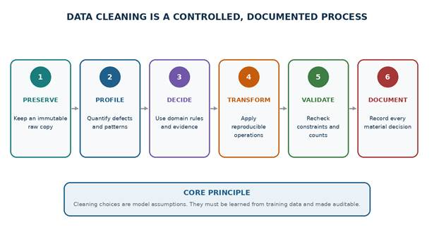
A practical, evidence-based chapter for turning imperfect raw records into a reliable modeling dataset while protecting evaluation integrity.
Chapter Overview
Real datasets are rarely clean. Values may be absent, duplicated, inconsistent, mistyped, measured in different units, or statistically unusual. Cleaning is therefore not a cosmetic step. Every correction, deletion, replacement, and transformation changes the information available to the model. The objective is not to make the table look perfect; it is to create a trustworthy representation of the problem while preserving traceability and preventing leakage.
KEY IDEA Cleaning is part of model design An imputation value, duplicate rule, category map, range constraint, or outlier treatment is an assumption about the data-generating process. Fit data-dependent choices on the training set and document their consequences. |
Learning objectives
- Differentiate explicit missing values, implicit missing values, structural absence, and censored values.
- Explain MCAR, MAR, and MNAR mechanisms and why they influence the validity of cleaning strategies.
- Quantify missingness by row, column, group, and pattern.
- Choose among deletion, simple imputation, missingness indicators, and model-based imputation.
- Detect exact duplicates, partial duplicates, duplicate entities, repeated measurements, and train-test overlap.
- Standardize labels, units, data types, ranges, and dates without destroying legitimate distinctions.
- Detect outliers using statistical and visual methods and decide whether to correct, retain, cap, transform, or model robustly.
- Build reproducible validation checks and a cleaning decision log.
- Apply cleaning operations in a pipeline that avoids leakage.
- Produce a documented, analysis-ready dataset and a defensible lab report.
Running dataset
Variable | Expected form | Injected defects | Role |
|---|---|---|---|
| record_id | Unique string | Duplicate records use repeated IDs | Traceability only |
| customer_id | Stable entity key | Some entities occur more than once | Grouping and duplicate checks |
| age | 18–100 years | Negative, child, and impossible values | Numerical feature |
| monthly_income | Monthly MAD | Missing values, annual values, extreme entries | Numerical feature |
| income_unit | MAD/month or MAD/year | Mixed units | Unit validation |
| city | Canonical city label | Case, spacing, spelling, and missing values | Categorical feature |
| plan | Basic, Plus, Premium | Case and trailing-space variants | Categorical feature |
| signup_date | Valid past ISO date | Impossible and future dates | Date feature |
| support_calls | Non-negative count | Missing values | Discrete feature |
| churned | 0 or 1 | Complete binary target | Target |
7.1 Missing Data
7.1.1 What counts as missing?
A value is missing when the dataset does not contain the information required by the variable definition. Missingness may be explicit—represented by NaN, NULL, None, or a blank—or implicit, hidden behind a sentinel such as -999, “unknown,” “not provided,” or an impossible date. A field can also be structurally absent: for example, pregnancy-related information may not apply to every patient. These cases should not automatically receive the same treatment.
Form | Example | Interpretation risk | First action |
|---|---|---|---|
| Explicit null | NaN, NULL, blank cell | Usually recognized by software | Confirm source meaning and frequency. |
| Sentinel value | -999, 9999, “N/A” | May be treated as a real value | Convert only after verifying the codebook. |
| Structural absence | End date for an active contract | Not an error; concept does not apply | Represent explicitly or derive a status flag. |
| Censored value | Income recorded as “>100,000” | Value is partially known | Preserve censoring information; do not use an arbitrary exact value. |
| Collection failure | Sensor offline | May be informative about conditions | Use process metadata and missingness indicators. |
| Not yet observed | Outcome label arrives after 30 days | Label delay rather than feature missingness | Define a label-maturity window. |
7.1.2 Missing-data mechanisms: MCAR, MAR, and MNAR
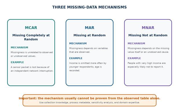
Figure 7.1 — Conceptual differences among MCAR, MAR, and MNAR missingness.
The mechanism describes why a value is missing, not merely how much is missing. Under MCAR, complete cases resemble incomplete cases on average. Under MAR, missingness can be explained by observed variables and may be addressed with conditional models. Under MNAR, the missing value or an unobserved factor influences missingness; standard imputation can remain biased. In practice, mechanisms are assumptions supported by collection knowledge and sensitivity analysis, not labels that can usually be proven from the table alone.
Mechanism | Formal intuition | Potential consequence | Example response |
|---|---|---|---|
| MCAR | P(M=1) independent of observed and missing values | Complete-case analysis can be unbiased but inefficient if the assumption holds. | Investigate random failures; quantify precision loss. |
| MAR | P(M=1) depends on observed variables | Conditional imputation can reduce bias when relevant predictors are included. | Impute within a pipeline using observed features. |
| MNAR | P(M=1) depends on the missing value or unobserved cause | Observed data alone may not identify the full distribution. | Use sensitivity analysis, external data, or explicit missingness models. |
CAUTION Do not diagnose mechanisms from percentages alone A column with 2% missing values may be MNAR, while a column with 40% may be structurally absent or MAR. Collection context matters more than the percentage. |
7.1.3 Missing-value percentages
Column-level percentages identify features with substantial missingness, but the denominator and scope must be stated. Calculate percentages on the appropriate dataset partition, retain raw counts, and examine whether missingness varies by time, source, target class, or observed subgroup.
PYTHON • EXAMPLE 7.1 — COLUMN-LEVEL MISSINGNESS SUMMARY import pandas as pd Keep both counts and percentages. A percentage without its denominator can be misleading. |
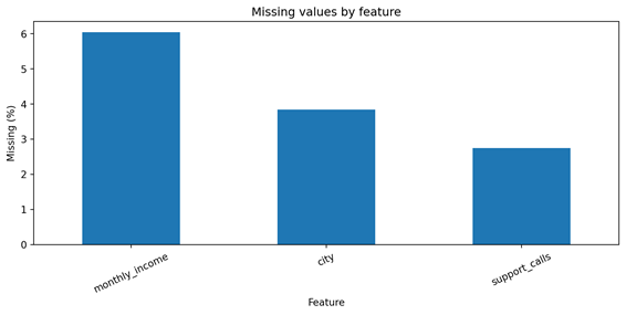
Figure 7.2 — Missingness in the deliberately imperfect laboratory dataset.
7.1.4 Rows versus columns with missing data
Column analysis asks whether a feature is usable. Row analysis asks whether individual observations contain enough information for a valid prediction or analysis. Removing a column can discard information from every observation; removing rows can distort the population if incomplete records differ systematically from complete records. The best decision often combines both perspectives.
PYTHON • EXAMPLE 7.2 — ROW-LEVEL MISSINGNESS BURDEN row_missing = df.isna().sum(axis=1) |
Question | Column perspective | Row perspective |
|---|---|---|
| How much information is absent? | Percentage missing in each feature | Number or percentage missing in each sample |
| What may be removed? | Feature if unusable or unavailable at inference | Observation if essential fields are absent |
| Main bias risk | Dropping a predictive but incomplete variable | Dropping a systematically different subgroup |
| Useful visualization | Missingness bar chart or matrix | Histogram of missing fields per row |
| Important extension | Missingness by group or time | Co-occurrence patterns across fields |
7.1.5 Missingness patterns and associations
Two variables may be missing together because they share a source system, form section, sensor, or process stage. Pattern analysis can reveal a pipeline failure or structural dependency that simple percentages hide. It is also useful to compare missingness with observed variables, while remembering that an association does not prove MAR or MNAR.
PYTHON • EXAMPLE 7.3 — MISSINGNESS INDICATORS AND GROUP COMPARISON df["income_missing"] = df["monthly_income"].isna().astype("int8") |
GOOD PRACTICE Target-aware inspection must be isolated During development, it can be useful to inspect whether feature missingness differs by target. Do this only inside the training data. The final test set must remain untouched until final evaluation. |
7.2 Missing-Value Strategies
There is no universally best strategy. The choice depends on the variable meaning, missingness mechanism, amount missing, sample size, algorithm, operational use, and cost of bias. A sound strategy begins by asking whether the value should exist, whether it can be recovered, and whether the absence itself contains information.
7.2.1 Strategy decision framework
Strategy | When it may be reasonable | Main risks | Pipeline requirement |
|---|---|---|---|
| Remove rows | Few rows are incomplete; missingness is plausibly MCAR; essential fields are absent | Loss of power and subgroup bias | Apply explicit rule before fitting or inside a documented transformer. |
| Remove feature | Feature is unavailable at prediction time, nearly empty, unreliable, or redundant | Discarding useful signal | Decide using training data and operational constraints. |
| Mean imputation | Roughly symmetric numeric feature; simple baseline | Reduces variance and weakens relationships | Fit mean on training data only. |
| Median imputation | Skewed numeric feature or moderate outliers | Still compresses distribution | Fit median on training data only. |
| Most-frequent imputation | Low-cardinality categorical feature with a dominant category | Overstates common category and hides uncertainty | Fit mode on training data only. |
| Constant imputation | Absence has a meaningful explicit state such as “Unknown” | May create an artificial cluster | Use a value distinguishable from real categories. |
| Missing indicator | Absence may carry process or behavioral information | Can encode undesirable collection bias | Generate consistently in train and inference. |
| Model-based imputation | Several observed variables predict the missing value | Complexity, overfitting, false precision | Fit imputer within cross-validation. |
| No imputation | Model handles missing values natively and semantics are acceptable | Behavior may be algorithm-specific | Validate performance and production compatibility. |
7.2.2 Removing rows
Complete-case analysis retains only rows without missing values in selected fields. It is easy to explain, but can waste information and alter the population. Define the subset of required variables explicitly; indiscriminately calling dropna() across the entire table can remove rows because of nonessential metadata.
PYTHON • EXAMPLE 7.4 — REMOVE ONLY ROWS MISSING ESSENTIAL FIELDS essential = ["customer_id", "churned"] |
COMMON MISTAKE Avoid blanket deletion `df.dropna()` may remove a record because an optional feature is missing. Name the fields, count the affected rows, and examine who is removed. |
7.2.3 Removing features
A high missing percentage is a warning, not an automatic deletion rule. A 70% complete laboratory biomarker may still be valuable if available at prediction time and measured for a meaningful subgroup. Conversely, a 99% complete post-event field must be removed because it leaks the target. Feature removal should combine data evidence with operational and domain requirements.
PYTHON • EXAMPLE 7.5 — FLAG FEATURES FOR REVIEW, NOT AUTOMATIC DELETION missing_pct = 100 * df.isna().mean() |
7.2.4 Mean and median imputation
Mean imputation preserves the observed mean of a symmetric variable but pulls missing records toward the center and underestimates variance. Median imputation is more robust to skew and extreme values. Both are simple baselines; neither recreates the uncertainty or conditional relationships of the missing observations.
PYTHON • EXAMPLE 7.6 — NUMERIC IMPUTATION IN A SCIKIT-LEARN PIPELINE from sklearn.impute import SimpleImputer |
7.2.5 Most-frequent and constant-value imputation
For categorical variables, the mode is convenient but can inflate the majority category. Constant imputation creates an explicit category such as “Unknown” or “Not recorded,” preserving the distinction between observed categories and missingness. Confirm that the chosen token cannot collide with a legitimate value.
PYTHON • EXAMPLE 7.7 — CATEGORICAL IMPUTATION from sklearn.impute import SimpleImputer |
7.2.6 Missing-value indicators
An indicator allows the model to distinguish an imputed value from a genuinely observed value. It is especially useful when the collection process carries information. However, the indicator may encode access, workflow, or demographic disparities. Its predictive value should be interpreted carefully and monitored over time.
PYTHON • EXAMPLE 7.8 — ADD INDICATORS AUTOMATICALLY from sklearn.impute import SimpleImputer The imputer learns medians and which columns need indicators from the training data only. |
7.2.7 Model-based imputation
Model-based methods estimate a missing feature using other observed variables. K-nearest-neighbor imputation uses similar rows; iterative imputation models each incomplete feature conditionally on other features. These methods can preserve relationships better than a constant statistic, but they add computational cost, may amplify bias, and can create an unjustified impression of precision.
PYTHON • EXAMPLE 7.9 — K-NEAREST-NEIGHBOR IMPUTATION from sklearn.impute import KNNImputer KNN distance is scale-sensitive. Evaluate the complete preprocessing design inside cross-validation. |
PYTHON • EXAMPLE 7.10 — ITERATIVE IMPUTATION from sklearn.experimental import enable_iterative_imputer # noqa: F401 |
7.2.8 When not to impute
- The value is structurally inapplicable and should be represented by a separate state or model design.
- The feature will not be available at prediction time; remove it rather than fabricate availability.
- The target is missing or immature; do not invent labels for supervised training without a defensible labeling method.
- The missingness mechanism is likely MNAR and a simple imputation would conceal major uncertainty.
- The variable is mostly missing, poorly defined, or unreliable and contributes little validated value.
- A native missing-value model has been validated and preserves a meaningful distinction.
- The imputation would violate physical constraints or produce an impossible combination.
- The downstream decision requires an actual measurement, not an estimated substitute.
COMMON MISTAKE Never impute the target casually Supervised models learn from labels. Filling missing targets with the majority class, a mean, or the model’s own predictions creates circular evidence and can invalidate evaluation. |
7.2.9 Compare strategies with cross-validation
Treat imputation as a hyperparameter of the modeling system. Compare plausible strategies using identical folds and a complete pipeline. The comparison should include performance, stability, calibration, subgroup effects, and operational interpretability—not only the mean score.
PYTHON • EXAMPLE 7.11 — COMPARE NUMERIC IMPUTATION STRATEGIES from sklearn.model_selection import cross_validate |
7.3 Duplicate Data
A duplicate is not defined only by identical rows. The relevant question is whether multiple records represent the same event, entity, measurement, or information. Some repetitions are legitimate longitudinal observations; others are accidental copies that distort frequencies and leak information across data splits.
7.3.1 Exact duplicates
Exact duplicates have identical values across the selected comparison columns. A technical identifier or ingestion timestamp may differ even when the substantive record is the same, so duplicate detection should explicitly exclude fields that are expected to be unique.
PYTHON • EXAMPLE 7.12 — DETECT EXACT SUBSTANTIVE DUPLICATES substantive_columns = [ |
7.3.2 Partial duplicates
Partial duplicates match on a meaningful key but disagree on one or more attributes. They may represent corrections, updates, concurrent records, or conflicts between sources. Do not keep an arbitrary first or last row until the ordering, source reliability, and business rule are understood.
Situation | Possible rule | Required evidence |
|---|---|---|
| Same transaction ID, identical business fields | Keep one record | Confirm accidental re-ingestion. |
| Same customer and timestamp, different amount | Investigate conflict | Source system, update sequence, or audit trail. |
| Same entity, different observation dates | Retain as repeated measurements | Ensure time is part of the unit of observation. |
| Same entity and date, corrected status | Keep latest valid version | Reliable version number or processing timestamp. |
| Near-match names and addresses | Potential duplicate entities | Entity-resolution method and human review for uncertain matches. |
PYTHON • EXAMPLE 7.13 — FIND REPEATED ENTITY-DATE KEYS key = ["customer_id", "signup_date"] |
7.3.3 Duplicate entities
A customer, patient, machine, or person can appear in several rows. Whether this is duplication depends on the unit of observation. If each row is a transaction, repeated customers are expected. If each row should represent one customer at a fixed prediction time, multiple rows require aggregation or a version-selection rule.
PYTHON • EXAMPLE 7.14 — COUNT OBSERVATIONS PER ENTITY entity_counts = df["customer_id"].value_counts(dropna=False) |
7.3.4 Repeated measurements
Repeated measurements can be valuable temporal information. Removing them as duplicates would destroy the signal. Instead, preserve the measurement timestamp, define the prediction index time, and create history features using only observations available before that time. Splitting should keep correlated measurements from the same entity together unless the evaluation explicitly simulates future observations of known entities.
Unit of observation | Repeated rows are… | Suitable split |
|---|---|---|
| One patient | Potential duplicates unless versions are intended | Group split by patient |
| One patient visit | Legitimate repeated measurements | Group or time-aware split |
| One machine cycle | Legitimate if cycle ID differs | Group by machine and consider time |
| One daily store record | Legitimate longitudinal observations | Time-based split |
| One transaction | Legitimate if transaction IDs differ | Group by customer if entity memorization is a risk |
7.3.5 Duplicate train-test records
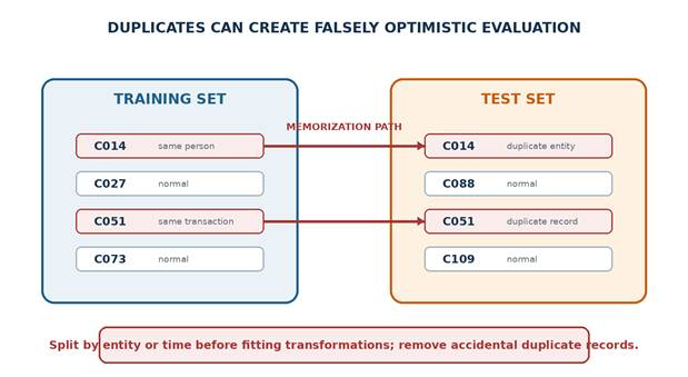
Figure 7.3 — Overlapping records or entities can turn evaluation into memorization.
If the same record appears in training and testing, the score no longer measures generalization. Even nonidentical rows from the same entity can leak stable identifiers, demographics, or behavior. Perform entity-aware or time-aware splitting before data-dependent preprocessing and verify overlap explicitly.
PYTHON • EXAMPLE 7.15 — VERIFY ENTITY SEPARATION AFTER SPLITTING train_entities = set(X_train["customer_id"]) |
7.3.6 Effects of duplication on evaluation
- Inflated accuracy because copied records are easy to recognize.
- Narrow confidence intervals because repeated rows are not independent evidence.
- Distorted class balance and category frequencies.
- Overweighting of entities with many accidental copies.
- Biased feature importance toward identifiers or stable entity characteristics.
- Unrealistic estimates of deployment performance on new entities or future periods.
- Potentially contradictory labels for the same substantive record.
- Unstable metrics when duplicate groups are distributed unevenly across folds.
GOOD PRACTICE Deduplication before or after splitting? Identify duplication rules using the raw data and domain definition. Remove accidental exact records before splitting, then use group-aware splitting for legitimate repeated entities. Fit learned cleaning parameters only on training folds. |
7.4 Inconsistent Data
Inconsistency occurs when values that should share a common meaning use different representations, units, types, or constraints. Standardization should improve semantic consistency without collapsing genuinely different categories. Preserve the raw field or an audit trail whenever transformations are material.
7.4.1 Typographical errors and inconsistent labels
Case, whitespace, punctuation, accents, abbreviations, and spelling can split one category into several levels. Begin with conservative normalization—trim whitespace and standardize case—then map verified variants to canonical values. Fuzzy matching should produce candidates for review rather than silently changing uncertain records.
PYTHON • EXAMPLE 7.16 — CONSERVATIVE CATEGORICAL NORMALIZATION city_map = { |
PYTHON • EXAMPLE 7.17 — VALIDATE CATEGORIES AGAINST AN ALLOWED SET allowed_plans = {"Basic", "Plus", "Premium"} |
7.4.2 Unit inconsistencies
A single numeric column can combine monthly and annual income, kilograms and pounds, Celsius and Fahrenheit, or seconds and milliseconds. Such values may look like outliers even though the measurements are valid. Convert to a canonical unit using a verified unit field or source-specific metadata, and retain the original value for traceability.
PYTHON • EXAMPLE 7.18 — CONVERT INCOME TO A CANONICAL MONTHLY UNIT def to_monthly_income(row): |
CAUTION Convert units before outlier deletion A value of 96,000 may be a valid annual salary rather than an impossible monthly value. Investigate units and source systems before applying statistical thresholds. |
7.4.3 Incorrect data types
Numeric values may be stored as text because of currency symbols, decimal separators, or mixed tokens. Dates may be generic strings. Boolean fields may use yes/no, 0/1, and true/false simultaneously. Convert explicitly, count failed conversions, and avoid silently coercing unexpected values to missing without an audit report.
PYTHON • EXAMPLE 7.19 — SAFE NUMERIC CONVERSION WITH FAILURE REPORTING raw_income = df["monthly_income_raw"].astype("string") |
7.4.4 Invalid ranges and impossible values
Range validation combines universal constraints and domain rules. Support-call counts cannot be negative. An age may be technically possible but incompatible with the target population. A transaction date may be valid in the calendar but occur before the system existed. Rules should distinguish hard impossibility from a review range.
Rule type | Example | Recommended handling |
|---|---|---|
| Hard physical/logical rule | support_calls < 0 | Reject, correct from source, or set missing with a logged reason. |
| Domain eligibility rule | age < 18 for an adult-only service | Investigate population definition and source record. |
| Plausibility review range | monthly income > 100,000 MAD | Review unit, source, and customer segment; do not auto-delete. |
| Cross-field constraint | end_date before start_date | Resolve temporal inconsistency or exclude the interval. |
| Conditional constraint | pregnancy_status present for inapplicable records | Review structural missingness and schema design. |
PYTHON • EXAMPLE 7.20 — REUSABLE VALIDATION ASSERTIONS rules = { |
7.4.5 Date inconsistencies
Date problems include ambiguous day-month order, impossible calendar dates, future dates, swapped fields, mixed time zones, and timestamps outside the observation window. Parse with an explicit expected format when possible, preserve failures, and validate dates relative to a clearly defined reference time.
PYTHON • EXAMPLE 7.21 — PARSE AND VALIDATE DATES reference_date = pd.Timestamp("2026-08-01") |
7.4.6 Cross-field and schema consistency
Individual values can be valid while their combination is impossible. Examples include a closure date before signup, a premium discount greater than the charge, or a newborn with 15 years of employment. Cross-field rules and schema checks should be encoded as executable tests so that new data can be rejected or quarantined automatically.
PYTHON • EXAMPLE 7.22 — CROSS-FIELD VALIDATION REPORT checks = pd.DataFrame(index=df.index) |
7.5 Outliers
7.5.1 Definition of an outlier
An outlier is an observation that is unusual relative to a reference distribution, rule, model, or domain expectation. The reference must be stated. A value can be globally unusual but normal within a subgroup, or numerically extreme but operationally important. Outlier detection produces candidates for investigation—not an automatic deletion list.
Type | Meaning | Example |
|---|---|---|
| Statistical outlier | Far from the bulk under a numerical rule | Income above Q3 + 1.5×IQR |
| Domain-specific outlier | Violates or approaches a domain expectation | Age 220 or negative sensor pressure |
| Measurement error | Generated by malfunction, entry error, or unit error | Temperature 900°C from a faulty sensor |
| Valid rare observation | Uncommon but real member of the population | A legitimate high-value transaction |
| Contextual outlier | Unusual only in a specific context | High energy use at night but normal during production |
| Collective anomaly | A sequence or group is unusual together | A gradual sensor drift across several measurements |
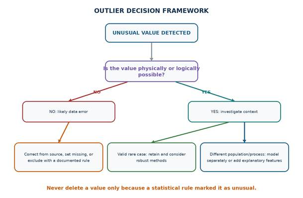
Figure 7.4 — A domain-informed decision process for unusual observations.
7.5.2 Z-score
The z-score measures distance from the mean in standard-deviation units: z = (x − μ) / σ. A common screening threshold is |z| > 3, but this is not a universal law. The method is sensitive to extreme values and is most interpretable for approximately symmetric distributions. Compute training statistics only, then apply them consistently to validation and test data.
PYTHON • EXAMPLE 7.23 — Z-SCORE CANDIDATES mean_income = X_train["monthly_income_clean"].mean() |
7.5.3 Interquartile range
The interquartile range is IQR = Q3 − Q1. Tukey fences commonly flag values below Q1 − 1.5×IQR or above Q3 + 1.5×IQR. The method is robust to extreme values but still depends on the population and distribution. For strongly skewed data, many valid tail observations may be flagged.
PYTHON • EXAMPLE 7.24 — IQR CANDIDATES series = X_train["monthly_income_clean"].dropna() |
7.5.4 Visual detection
Histograms, box plots, scatter plots, and time-series plots reveal context that a threshold cannot. A box plot shows tail candidates but not sample density; a histogram shows shape but can hide relationships; a scatter plot can expose conditional anomalies; a time plot can identify spikes, drift, or sensor resets.
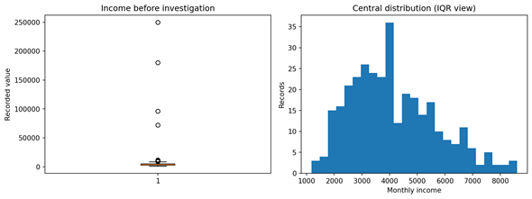
Figure 7.5 — Statistical candidates require contextual investigation before treatment.
PYTHON • EXAMPLE 7.25 — COMPLEMENTARY VISUAL CHECKS import matplotlib.pyplot as plt |
7.5.5 Capping and transformation
Capping limits values to selected bounds, often training quantiles. It can reduce the influence of extreme values but changes legitimate observations and creates a pile-up at the boundary. Log or power transformations compress positive skew while retaining order. Both operations must be justified, fitted on training data, and included in the reproducible pipeline.
PYTHON • EXAMPLE 7.26 — TRAINING-DERIVED QUANTILE CAPPING lower, upper = X_train["monthly_income_clean"].quantile([0.01, 0.99]) The bounds come only from training data. Record the percentage capped in every partition. |
PYTHON • EXAMPLE 7.27 — LOG TRANSFORMATION FOR POSITIVE SKEW import numpy as np |
7.5.6 Robust models and robust statistics
Sometimes the best response is to keep valid extremes and choose methods that are less sensitive to them. Median and IQR summaries, RobustScaler, Huber regression, quantile regression, and tree-based models can reduce influence without deleting observations. Robustness does not eliminate the need to fix impossible values or unit errors.
PYTHON • EXAMPLE 7.28 — ROBUST SCALING AND HUBER REGRESSION from sklearn.pipeline import Pipeline |
CAUTION Rare cases may be the objective Fraud, equipment failure, severe disease, and cyberattacks are intentionally rare. Removing unusual target-positive cases can destroy the problem the model is meant to solve. |
Practical Lab — Clean a Deliberately Imperfect Dataset
PRACTICAL LAB Lab objective Create an auditable cleaning workflow that preserves raw data, diagnoses defects, applies justified transformations, validates the result, and protects the test set. |
Scenario
A subscription company wants to train a churn classifier. The extracted table contains missing values, exact duplicates, repeated customer entities, category variants, mixed income units, invalid ages, malformed dates, and extreme income values. Students must create a cleaning notebook and document every decision. The target is churned; each modeling observation should represent one customer snapshot.
Required outputs
- An immutable raw-data object and a separate working copy.
- A data-quality audit with counts, percentages, examples, and affected identifiers.
- A written cleaning decision log containing evidence, rule, action, and impact.
- A cleaned feature table with documented types and units.
- A duplicate and entity-overlap report.
- A missing-value strategy fitted only on training data.
- An outlier candidate report distinguishing errors from valid rare cases.
- Executable validation checks that fail when constraints are violated.
- A before-and-after summary of row count, entity count, missingness, and ranges.
- A short reflection on remaining uncertainty and model risks.
Lab Step 1 — Load and preserve the raw data
PYTHON • LAB 7.1 — LOAD WITHOUT OVERWRITING THE RAW TABLE from pathlib import Path |
Lab Step 2 — Build a compact audit
PYTHON • LAB 7.2 — DATA-QUALITY AUDIT FUNCTION def quality_audit(data, entity_key="customer_id"): |
Lab Step 3 — Create a decision log
Issue | Evidence | Decision rule | Action | Impact to record |
|---|---|---|---|---|
| Missing income | 22 rows; varies by plan | Retain rows; median imputation + indicator in training pipeline | Leave as NaN in cleaned table | Rows affected; validation score comparison |
| Exact duplicate records | Two complete copies | Same substantive fields and no version meaning | Keep one; preserve removed IDs in log | Rows removed; class balance before/after |
| Mixed income units | Two rows marked MAD/year | Unit metadata is trusted | Divide annual values by 12 | Original and converted values |
| Invalid ages | -4, 9, 220 | Adult service: valid range 18–100 | Set to missing and flag source error | IDs and original values |
| Category variants | Case, spaces, Tanger/Tangier | Verified canonical map | Normalize to approved labels | Unmapped values must be zero |
| Malformed/future dates | Impossible and future strings | Date must parse and be ≤ reference date | Set missing; create issue flag | IDs, original text, reason |
| High income | Some annual units; two extreme monthly values | Correct units first, then review domain evidence | Retain valid high values; compare robust methods | Candidate list and decision rationale |
Lab Step 4 — Normalize text and units
PYTHON • LAB 7.3 — CANONICALIZATION FUNCTIONS CITY_MAP = { |
Lab Step 5 — Validate and quarantine impossible values
PYTHON • LAB 7.4 — APPLY EXPLICIT HARD CONSTRAINTS reference_date = pd.Timestamp("2026-08-01") |
Lab Step 6 — Resolve exact duplicates and preserve entity groups
PYTHON • LAB 7.5 — REMOVE ACCIDENTAL COPIES substantive = [ |
The two remaining repeated customers have different support-call values. They are not automatically deleted. Because the project defines one customer snapshot, the team must identify the correct version using a reliable timestamp or source rule. If no defensible rule exists, quarantine the conflicting entities rather than selecting a row arbitrarily.
Lab Step 7 — Split by entity before fitting imputers
PYTHON • LAB 7.6 — GROUP-AWARE TRAIN-TEST SPLIT from sklearn.model_selection import GroupShuffleSplit |
Lab Step 8 — Build leakage-safe preprocessing
PYTHON • LAB 7.7 — NUMERIC AND CATEGORICAL PIPELINES from sklearn.compose import ColumnTransformer |
Lab Step 9 — Validate the cleaned result
PYTHON • LAB 7.8 — ASSERTIONS AND BEFORE-AFTER COMPARISON assert working["churned"].isin([0, 1]).all() |
Lab Step 10 — Document five cleaning decisions
For each decision, students write a concise paragraph containing: the evidence, the rule, the action, the number of affected records, the expected modeling consequence, and any remaining uncertainty. The following is a model statement:
GOOD PRACTICE Example evidence-based decision Two records contained income values of 72,000 and 96,000 with the unit “MAD/year.” They were converted to 6,000 and 8,000 MAD/month using the trusted unit field. No rows were removed. The original values and units were retained in the audit table. This conversion was performed before outlier screening because mixed units would otherwise create false anomaly candidates. |
Lab deliverable checklist
Deliverable component | Minimum evidence |
|---|---|
| Dataset dimensions | Rows, columns, unique entities before and after cleaning |
| Missing-data report | Counts, percentages, row burden, and chosen strategy by feature |
| Duplicate report | Exact copies, repeated keys, entity counts, and split-overlap assertion |
| Consistency report | Category map, unit conversions, type failures, range and date rules |
| Outlier report | Candidate method, IDs, domain investigation, and final action |
| Decision log | Evidence, rule, action, impact, and responsible reviewer |
| Reproducibility | Notebook runs top-to-bottom; fixed random state; no hidden manual edits |
| Leakage protection | Group-aware split; all learned transformations fitted on training data |
| Validation | Assertions pass; unexpected categories and rule failures are reported |
| Reflection | Remaining uncertainty, possible bias, and next data-collection improvements |
Worked Mini-Cases
Case 1 — Medical measurement missing after device failure
A blood-pressure field is missing for 8% of visits. Missingness is concentrated at one clinic during a device outage. This is related to an observed site and time period, so a MAR assumption may be plausible if clinic and date are included. A complete-case deletion could remove an entire operational episode. A pipeline-based imputation with clinic/time predictors, a missingness indicator, and a clinic-specific sensitivity analysis is more defensible.
Case 2 — Rare fraudulent transactions
Large transactions are flagged by an IQR rule. Investigation shows that several are confirmed fraud and several are legitimate business purchases. Deleting all flagged rows would remove target-positive examples and high-value legitimate cases. The team retains them, corrects one currency conversion error, applies robust scaling, and evaluates precision-recall performance by transaction-value range.
Case 3 — Duplicate patient records
Two hospitals contribute records for the same patient. Names differ slightly and local IDs are different. Fuzzy matching is used only to generate candidate pairs; uncertain matches are reviewed. Confirmed duplicate entities are assigned a stable cross-source patient ID. All visits are retained, but group cross-validation ensures that the same patient never occurs in both training and validation folds.
Knowledge Check
1. Explain why a high percentage of missing values does not automatically justify dropping a feature.
2. Differentiate MCAR, MAR, and MNAR using one original example for each mechanism.
3. Why should imputation statistics be fitted only on the training data?
4. When can repeated rows be valid rather than duplicates?
5. Why may exact duplicate records inflate a test score?
6. Describe one risk of most-frequent categorical imputation.
7. Why should unit conversion occur before statistical outlier detection?
8. Compare z-score and IQR screening.
9. Give two situations in which a statistically extreme observation should be retained.
10. What information belongs in a cleaning decision log?
11. Why is fuzzy matching unsuitable as an automatic deletion rule?
12. What is the difference between an impossible value and a valid rare value?
Suggested Answers
Question | Suggested answer |
|---|---|
| 1 | Missingness percentage does not reveal feature importance, mechanism, subgroup coverage, operational availability, or whether absence is structural. Review meaning and predictive value. |
| 2 | MCAR: independent packet loss. MAR: survey income missing more often among an observed age group. MNAR: high earners are more likely to omit income because of the value itself. |
| 3 | Using validation or test values changes the learned statistic and leaks information about the evaluation distribution, producing optimistic or nonreproducible estimates. |
| 4 | Repeated rows are valid when the unit is a visit, transaction, cycle, or time point and each row represents a distinct event. |
| 5 | The model may memorize a record seen during training, so the test result measures recognition rather than generalization. |
| 6 | It inflates the dominant category, hides uncertainty, and can distort class-conditional relationships. |
| 7 | Mixed units generate false extremes. Canonical units are required before values can be compared meaningfully. |
| 8 | Z-scores use mean and standard deviation and are sensitive to extremes; IQR fences use quartiles and are more robust, but both are context-dependent screens. |
| 9 | Retain a confirmed rare customer or a true fraud/failure case; retain an extreme value that is valid within a particular subgroup. |
| 10 | Evidence, affected records, decision rule, action, impact, reviewer, date/version, and unresolved uncertainty. |
| 11 | Similarity scores can merge different people or events. Candidate matches require thresholds, supporting fields, and review for uncertain cases. |
| 12 | An impossible value violates a hard logical or physical rule; a valid rare value is possible and confirmed, even if statistically unusual. |
Chapter Summary
- Missingness must be interpreted through variable meaning, collection process, and mechanism—not percentage alone.
- Rows and columns provide complementary views of missing data; deletion can introduce bias.
- Imputation changes distributions and relationships. Fit all data-dependent choices on training data.
- Exact copies, conflicting keys, duplicate entities, and legitimate repeated measurements require different rules.
- Train-test overlap invalidates generalization estimates; use entity- or time-aware splitting when necessary.
- Label, unit, type, range, and date consistency should be enforced with explicit, executable rules.
- Outlier methods identify candidates. Domain evidence determines whether to correct, retain, transform, cap, or exclude.
- Robust methods can reduce sensitivity to valid extremes without deleting valuable information.
- Every material cleaning decision should be reproducible, auditable, and linked to affected records.
- A clean dataset is not one with no missing values or extreme observations; it is one whose limitations and transformations are understood.
Key Terms
Term | Meaning |
|---|---|
| MCAR | Missingness unrelated to observed and unobserved values. |
| MAR | Missingness explained by observed variables, under an assumption. |
| MNAR | Missingness related to the missing value or an unobserved cause. |
| Imputation | Replacement or estimation of missing feature values. |
| Missingness indicator | Binary feature showing whether the original value was absent. |
| Exact duplicate | Repeated substantive record with identical compared fields. |
| Duplicate entity | Multiple records referring to the same real-world entity. |
| Entity leakage | The same entity contributes information to training and evaluation sets. |
| Canonical value | Approved representation used for a semantic category or unit. |
| Hard constraint | Rule that defines physical or logical impossibility. |
| Outlier | Observation unusual relative to a stated reference. |
| IQR | Difference between the third and first quartiles. |
| Capping | Replacing values outside selected bounds with the boundary values. |
| Robust method | Method designed to reduce sensitivity to extreme observations. |
| Decision log | Audit record explaining evidence, rule, action, and impact of a cleaning choice. |
DEFINITION Expected outcome Students can transform an imperfect dataset into an analysis-ready training resource while preserving raw evidence, preventing leakage, validating constraints, and documenting every consequential decision. |