Chapter 14 — Logistic Regression
| Chapter purpose This chapter develops logistic regression as a complete classification model: from the linear decision function and sigmoid probability transformation to thresholds, multiclass extensions, regularization, coefficient interpretation, and practical evaluation. The emphasis is on understanding both what the model computes and how to train it safely in scikit-learn. |
Learning objectives
- Explain why logistic regression is a classification model despite the word “regression” in its name.
- Compute and interpret the linear score, sigmoid probability, and class decision.
- Distinguish probabilities from final class labels and explain the role of a decision threshold.
- Interpret coefficient signs, magnitudes, log-odds, and odds ratios.
- Use logistic regression for binary and multiclass classification.
- Explain L1 and L2 regularization and the role of the scikit-learn parameter C.
- Build a leakage-safe training pipeline with scaling and logistic regression.
- Evaluate coefficients, probabilities, thresholds, and performance metrics in a practical lab.
| Key idea Logistic regression first computes a linear score and then transforms that score into a probability. Classification occurs only after a decision rule—usually a probability threshold—is applied. |
14.1 Logistic regression concepts
Logistic regression is one of the most important supervised classification algorithms. It is fast, statistically well understood, easy to regularize, and often an excellent baseline for tabular classification problems. Its simplicity is also useful for interpretation: each coefficient describes how one feature changes the model’s log-odds, holding the other features fixed.
Linear decision function
For a feature vector x = (x₁, x₂, …, xₚ), logistic regression begins with a weighted linear combination of the input features. The intercept β₀ shifts the decision function, while each coefficient βⱼ controls the contribution of feature xⱼ.
z = β₀ + β₁x₁ + β₂x₂ + ··· + βₚxₚ
The quantity z is not yet a probability. It can take any real value from negative infinity to positive infinity. Large positive values indicate stronger evidence for the positive class, while large negative values indicate stronger evidence for the negative class.
Python 14.1 — Computing the linear decision score
| import numpy as np # Example: z = intercept + b1*x1 + b2*x2 intercept = -2.0 coef = np.array([0.7, -0.4]) x = np.array([3.0, 1.5]) z = intercept + x @ coef print(f'Linear score z = {z:.3f}') |
Probability prediction and the sigmoid function
To obtain a value between 0 and 1, logistic regression passes z through the sigmoid, also called the logistic function. This produces the estimated probability of the positive class.
P(y = 1 | X) = 1 / (1 + e^(−z))
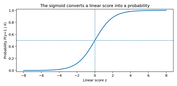
Figure 14.1 — Sigmoid transformation from the linear score z to a probability.
The sigmoid is monotonic: increasing z always increases the probability. At z = 0, the probability is exactly 0.5. Very negative scores approach 0, while very positive scores approach 1. The model therefore retains a linear structure in z while producing valid probabilities.
Python 14.2 — Implementing the sigmoid function
| import numpy as np def sigmoid(z): return 1 / (1 + np.exp(-z)) for z in [-3, -1, 0, 1, 3]: print(z, '->', round(sigmoid(z), 4)) |
Log-odds and odds interpretation
Logistic regression is linear in the log-odds rather than directly in probability. If p is the probability of the positive class, the odds are p/(1−p), and the logit is the natural logarithm of those odds.
log(p / (1 − p)) = β₀ + β₁x₁ + ··· + βₚxₚ
A one-unit increase in xⱼ changes the log-odds by βⱼ. Exponentiating the coefficient gives an odds ratio, exp(βⱼ). An odds ratio greater than 1 increases the odds of the positive class; a value below 1 decreases them.
Coefficient | exp(coefficient) | Interpretation for a +1 feature change |
|---|---|---|
| β = 0.00 | 1.00 | No change in odds. |
| β = 0.40 | 1.49 | Odds multiply by about 1.49. |
| β = 0.69 | 1.99 | Odds approximately double. |
| β = −0.40 | 0.67 | Odds multiply by about 0.67. |
| β = −0.69 | 0.50 | Odds are approximately halved. |
| Interpretation caution A coefficient describes association in the fitted predictive model. It is not automatically a causal effect. Correlated features, omitted variables, encoding choices, scaling, and data-collection processes all affect coefficient interpretation. |
Decision threshold and class prediction
Probabilities and class predictions are different outputs. A classifier converts probability into a label by comparing it with a threshold. The conventional binary threshold is 0.5, but the threshold should reflect the application’s error costs and operating requirements.
ŷ = 1 if P(y = 1 | X) ≥ threshold; otherwise ŷ = 0
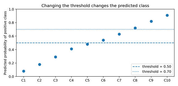
Figure 14.2 — A higher threshold produces fewer positive predictions.
Python 14.3 — Converting probabilities into class labels
| probabilities = np.array([0.18, 0.41, 0.54, 0.72, 0.91]) pred_05 = (probabilities >= 0.50).astype(int) pred_07 = (probabilities >= 0.70).astype(int) print('threshold 0.50:', pred_05) print('threshold 0.70:', pred_07) |
Coefficients and feature effects
For numerical features, the coefficient sign indicates whether increasing the feature tends to increase or decrease the positive-class log-odds. Magnitude should be interpreted carefully because coefficients are measured per feature unit. Scaling numerical variables can make coefficient magnitudes easier to compare.
Coefficient sign | Effect on z | Effect on positive-class probability |
|---|---|---|
| Positive | z increases as the feature increases | Probability tends to increase. |
| Negative | z decreases as the feature increases | Probability tends to decrease. |
| Near zero | Small linear contribution | Little linear predictive contribution, conditional on other features. |
Python 14.4 — Inspecting coefficients and odds ratios
| import pandas as pd coef_table = pd.DataFrame({ 'feature': feature_names, 'coefficient': model.coef_[0] }) coef_table['odds_ratio'] = np.exp(coef_table['coefficient']) coef_table = coef_table.sort_values('coefficient', ascending=False) print(coef_table) |
14.2 Binary classification
Binary classification contains two mutually exclusive classes. Examples include churn/no churn, defective/not defective, approved/not approved, and response/no response. Logistic regression models the probability of one class—typically encoded as 1—relative to the other class, usually encoded as 0.
Positive and negative classes
The terms positive and negative do not imply good and bad. They are simply roles assigned during evaluation. The positive class is usually the event of primary interest, such as fraud, churn, failure, or purchase. Correctly defining the positive class is important because precision, recall, and threshold decisions are expressed relative to it.
Actual / Predicted | Predicted 0 | Predicted 1 |
|---|---|---|
| Actual 0 | True negative (TN) | False positive (FP) |
| Actual 1 | False negative (FN) | True positive (TP) |
Probability outputs
scikit-learn LogisticRegression exposes predict_proba(). In binary classification it returns two columns: P(y=0|X) and P(y=1|X). Each row sums to 1. The positive-class probability is commonly the second column when classes_ is [0, 1].
Python 14.5 — Obtaining class probabilities
| from sklearn.linear_model import LogisticRegression model = LogisticRegression(max_iter=1000) model.fit(X_train, y_train) prob_matrix = model.predict_proba(X_test) print('Class order:', model.classes_) print('First probability pair:', prob_matrix[0]) p_positive = prob_matrix[:, 1] |
Threshold of 0.5
The default 0.5 threshold is natural when the model is reasonably calibrated and the costs of false positives and false negatives are similar. It is not a universal optimum. Business capacity, risk tolerance, intervention cost, and class imbalance may justify another threshold.
Python 14.6 — Verifying the default 0.5 decision rule
| # scikit-learn's default hard predictions pred_default = model.predict(X_test) # Equivalent manual rule for binary classes 0 and 1 p_positive = model.predict_proba(X_test)[:, 1] pred_manual = (p_positive >= 0.5).astype(int) print((pred_default == pred_manual).all()) |
Changing the decision threshold
Lowering the threshold generally increases the number of positive predictions. This often increases recall but can reduce precision. Raising the threshold generally does the opposite. Threshold selection should therefore be separated conceptually from model training: the same fitted probability model can support different operating points.
Threshold change | Positive predictions | Typical recall effect | Typical precision effect |
|---|---|---|---|
| Lower threshold | More | Increases | May decrease |
| Higher threshold | Fewer | Decreases | May increase |
Python 14.7 — Comparing several thresholds
| from sklearn.metrics import precision_score, recall_score, f1_score p = model.predict_proba(X_test)[:, 1] for threshold in [0.30, 0.50, 0.70]: pred = (p >= threshold).astype(int) print( threshold, 'precision=', round(precision_score(y_test, pred), 3), 'recall=', round(recall_score(y_test, pred), 3), 'f1=', round(f1_score(y_test, pred), 3) ) |
| Operational example Suppose a retention team can contact only 500 customers per week. The model may rank customers by churn probability, and the operating threshold can be chosen so that approximately 500 customers are flagged. This is different from assuming 0.5 is automatically best. |
Decision function versus probability
LogisticRegression also provides decision_function(), which returns the linear score z. Because the sigmoid is monotonic, ranking examples by z produces the same ordering as ranking by positive-class probability. Probability is easier to communicate; the decision score is useful for understanding margins and threshold equivalence.
Python 14.8 — Connecting decision scores and probabilities
| z = model.decision_function(X_test) p = model.predict_proba(X_test)[:, 1] # Convert z manually to a probability p_from_z = 1 / (1 + np.exp(-z)) print(np.allclose(p, p_from_z)) |
14.3 Multiclass classification
When the target contains more than two classes, logistic regression can be extended to multiclass classification. The output becomes a probability distribution over all classes, and the predicted class is normally the class with the highest estimated probability.
One-versus-rest
One-versus-rest (OvR) trains one binary classifier per class. For class k, observations from class k are treated as positive and all other classes as negative. At prediction time, the class with the strongest score is selected. OvR is conceptually simple and works with many binary classifiers.
Classifier | Positive class | Negative class |
|---|---|---|
| Model 1 | Class A | Classes B and C |
| Model 2 | Class B | Classes A and C |
| Model 3 | Class C | Classes A and B |
Multinomial logistic regression
Multinomial logistic regression models all classes jointly. It uses a softmax transformation so that the class probabilities are non-negative and sum to 1. This joint formulation is often preferable when classes are mutually exclusive and the chosen solver supports multinomial optimization.
P(y = k | X) = exp(zₖ) / Σⱼ exp(zⱼ)
Python 14.9 — Training a multiclass logistic-regression pipeline
| from sklearn.datasets import load_iris from sklearn.model_selection import train_test_split from sklearn.preprocessing import StandardScaler from sklearn.pipeline import Pipeline from sklearn.linear_model import LogisticRegression X, y = load_iris(return_X_y=True) X_train, X_test, y_train, y_test = train_test_split( X, y, test_size=0.25, random_state=42, stratify=y ) multi_model = Pipeline([ ('scale', StandardScaler()), ('logreg', LogisticRegression(max_iter=1000)) ]) multi_model.fit(X_train, y_train) |
Class probabilities
For K classes, predict_proba() returns K probabilities per observation. The classes_ attribute defines the column order. Always inspect classes_ instead of assuming that a particular class corresponds to a particular column.
Python 14.10 — Inspecting multiclass probability vectors
| probs = multi_model.predict_proba(X_test[:3]) classes = multi_model.named_steps['logreg'].classes_ print('Classes:', classes) print('Probability matrix: ', probs) print('Row sums:', probs.sum(axis=1)) |
| Important In multiclass problems, probability interpretation depends on the training formulation, solver, regularization, and calibration. A probability vector is useful, but it should still be validated before it is treated as a precise real-world risk estimate. |
14.4 Regularization
Regularization controls coefficient magnitude and helps reduce overfitting. Logistic regression normally optimizes a data-fitting objective plus a penalty. Stronger regularization discourages very large coefficients, which can improve stability when features are noisy, correlated, numerous, or measured on different scales.
L2 regularization
L2 regularization penalizes the squared magnitude of coefficients. It tends to shrink coefficients smoothly toward zero but usually does not make them exactly zero. L2 is a strong default choice because it is stable when predictors are correlated and is supported by common solvers.
Penalty(L2) = λ Σⱼ βⱼ²
- Shrinks all coefficients continuously.
- Often improves stability when features are correlated.
- Usually retains every input feature in the fitted model.
L1 regularization
L1 regularization penalizes the absolute magnitude of coefficients. It can force some coefficients exactly to zero, which gives it an embedded feature-selection effect. This can produce a sparse model, although the selected features may be unstable when several predictors contain similar information.
Penalty(L1) = λ Σⱼ |βⱼ|
- Can produce exact zero coefficients.
- Useful when sparse solutions are desirable.
- Requires a solver that supports L1, such as liblinear for suitable binary settings or saga for broader cases.
Regularization strength and the parameter C
In scikit-learn LogisticRegression, C is the inverse of regularization strength. This direction is easy to confuse: small C means strong regularization, while large C means weak regularization.
C value | Regularization | Typical effect |
|---|---|---|
| Very small, e.g. 0.01 | Strong | Coefficients strongly shrunk; possible underfitting. |
| Moderate, e.g. 1 | Default-scale reference | Balanced starting point; must still be validated. |
| Large, e.g. 100 | Weak | Model follows training data more closely; overfitting risk can rise. |
Python 14.11 — Observing how C changes coefficient magnitude
| from sklearn.linear_model import LogisticRegression for C in [0.01, 0.1, 1, 10, 100]: model = LogisticRegression(C=C, max_iter=1000) model.fit(X_train_scaled, y_train) print(C, np.linalg.norm(model.coef_)) |
Preventing overfitting
Regularization is most useful when its strength is selected on validation data or through cross-validation. The test set should remain untouched until the model, preprocessing, threshold strategy, and hyperparameters have been finalized. Regularization cannot compensate for leakage or a poor split strategy.
Python 14.12 — Tuning regularization safely inside a pipeline
| from sklearn.model_selection import GridSearchCV, StratifiedKFold param_grid = { 'logreg__C': [0.01, 0.1, 1, 10, 100] } cv = StratifiedKFold(n_splits=5, shuffle=True, random_state=42) search = GridSearchCV( pipeline, param_grid=param_grid, scoring='roc_auc', cv=cv ) search.fit(X_train, y_train) print(search.best_params_) |
Feature-selection effects of L1
When L1 regularization is strong enough, some fitted coefficients become exactly zero. This can simplify the model and highlight a subset of predictive variables, but zero does not mean a feature is scientifically irrelevant. Correlated alternatives may cause the algorithm to keep one feature and suppress another.
Python 14.13 — Inspecting sparsity created by L1
| l1_model = LogisticRegression( penalty='l1', solver='liblinear', C=0.2, max_iter=1000 ) l1_model.fit(X_train_scaled, y_train) coef = l1_model.coef_[0] print('Non-zero coefficients:', np.count_nonzero(coef)) print('Zero coefficients:', np.sum(coef == 0)) |
Why scaling matters
Regularization acts on coefficient magnitude. If one feature is measured in thousands and another in fractions, their coefficient scales are not directly comparable. Standardizing numerical features makes the penalty operate more evenly and is especially important for regularized linear models.
| Best practice For numerical tabular data, combine StandardScaler and LogisticRegression in a Pipeline. This prevents preprocessing leakage and ensures the same transformation is applied at training and prediction time. |
Python 14.14 — Scaling and logistic regression in one pipeline
| from sklearn.pipeline import Pipeline from sklearn.preprocessing import StandardScaler from sklearn.linear_model import LogisticRegression pipeline = Pipeline([ ('scale', StandardScaler()), ('logreg', LogisticRegression(C=1.0, max_iter=1000)) ]) pipeline.fit(X_train, y_train) |
14.5 Advantages and limitations
Advantages
Advantage | Why it matters |
|---|---|
| Fast | Training and prediction are efficient for many tabular datasets. |
| Interpretable | Coefficients, log-odds, and odds ratios provide a clear linear explanation. |
| Strong baseline | Often competitive when the relationship is approximately linear in the log-odds. |
| Probability output | predict_proba() supports ranking, thresholding, and expected-cost decisions. |
| Regularization | L1 and L2 provide direct control over model complexity. |
| Multiclass support | The model extends naturally to multiple mutually exclusive classes. |
Limitations
Limitation | Consequence / response |
|---|---|
| Linear decision boundary | Complex nonlinear patterns require engineered features or another model family. |
| Sensitive to feature scale under regularization | Scale numerical predictors in a leakage-safe pipeline. |
| Limited automatic interaction modeling | Interactions must be engineered explicitly if scientifically justified. |
| Sensitive to severe multicollinearity for interpretation | Coefficient signs and magnitudes can become unstable. |
| Outliers / extreme leverage can matter | Inspect data quality and consider robust preprocessing. |
| Probability calibration is not guaranteed | Evaluate calibration when probabilities drive important decisions. |
Linear decision boundary
In the original feature space, binary logistic regression separates classes using a hyperplane. The sigmoid changes the score into a probability but does not make the boundary nonlinear. Nonlinear behavior can be introduced through transformations, polynomial terms, splines, or interaction features, but excessive feature engineering can increase complexity and overfitting.
Python 14.15 — Adding nonlinear feature terms while keeping a linear classifier
| from sklearn.preprocessing import PolynomialFeatures from sklearn.pipeline import Pipeline nonlinear_logreg = Pipeline([ ('poly', PolynomialFeatures(degree=2, include_bias=False)), ('scale', StandardScaler()), ('logreg', LogisticRegression(max_iter=1000)) ]) |
Practical lab — Train and analyze a logistic regression classifier
In this lab, students build a binary classifier on a synthetic customer-renewal dataset. The goal is not only to obtain a score, but also to inspect probabilities, coefficients, threshold behavior, and multiple performance metrics.
Lab objectives
- Create a reproducible binary classification dataset.
- Create a stratified train/test split.
- Build a StandardScaler + LogisticRegression pipeline.
- Evaluate default 0.5-threshold predictions.
- Inspect positive-class probabilities.
- Compare several thresholds.
- Extract standardized coefficients and odds ratios.
- Interpret the model’s strengths and limitations.
Step 1 — Create the dataset
Python Lab 14.1 — Generate a reproducible classification dataset
| import pandas as pd from sklearn.datasets import make_classification X, y = make_classification( n_samples=1600, n_features=8, n_informative=5, n_redundant=1, weights=[0.68, 0.32], class_sep=1.1, random_state=42 ) feature_names = [ 'usage', 'support_calls', 'tenure', 'monthly_fee', 'engagement', 'late_payments', 'discount', 'service_score' ] X = pd.DataFrame(X, columns=feature_names) y = pd.Series(y, name='will_not_renew') print(X.head()) print(y.value_counts(normalize=True)) |
Step 2 — Split the data
Python Lab 14.2 — Stratified train/test split
| from sklearn.model_selection import train_test_split X_train, X_test, y_train, y_test = train_test_split( X, y, test_size=0.25, random_state=42, stratify=y ) print(X_train.shape, X_test.shape) print(y_train.mean(), y_test.mean()) |
Step 3 — Build and train the pipeline
Python Lab 14.3 — Train a scaled logistic regression model
| from sklearn.pipeline import Pipeline from sklearn.preprocessing import StandardScaler from sklearn.linear_model import LogisticRegression model = Pipeline([ ('scale', StandardScaler()), ('logreg', LogisticRegression(C=1.0, max_iter=1000)) ]) model.fit(X_train, y_train) |
Step 4 — Evaluate the default classifier
Python Lab 14.4 — Evaluate performance at the default threshold
| from sklearn.metrics import ( accuracy_score, precision_score, recall_score, f1_score, roc_auc_score, confusion_matrix ) pred = model.predict(X_test) prob = model.predict_proba(X_test)[:, 1] print('Accuracy :', round(accuracy_score(y_test, pred), 3)) print('Precision:', round(precision_score(y_test, pred), 3)) print('Recall :', round(recall_score(y_test, pred), 3)) print('F1 :', round(f1_score(y_test, pred), 3)) print('ROC AUC :', round(roc_auc_score(y_test, prob), 3)) print('Confusion matrix: ', confusion_matrix(y_test, pred)) |
Step 5 — Inspect probability predictions
Python Lab 14.5 — Rank observations by positive-class probability
| results = X_test.copy() results['actual'] = y_test.values results['p_positive'] = prob results['pred_0_50'] = pred print(results[['actual', 'p_positive', 'pred_0_50']] .sort_values('p_positive', ascending=False) .head(10)) |
Step 6 — Compare thresholds
Python Lab 14.6 — Build a threshold comparison table
| rows = [] for threshold in [0.30, 0.40, 0.50, 0.60, 0.70]: pred_t = (prob >= threshold).astype(int) rows.append({ 'threshold': threshold, 'precision': precision_score(y_test, pred_t), 'recall': recall_score(y_test, pred_t), 'f1': f1_score(y_test, pred_t), 'positive_predictions': pred_t.sum() }) threshold_table = pd.DataFrame(rows) print(threshold_table.round(3)) |
Step 7 — Analyze coefficients
Python Lab 14.7 — Interpret standardized coefficients and odds ratios
| import numpy as np logreg = model.named_steps['logreg'] coef_table = pd.DataFrame({ 'feature': feature_names, 'coefficient': logreg.coef_[0] }) coef_table['odds_ratio'] = np.exp(coef_table['coefficient']) coef_table['abs_coefficient'] = coef_table['coefficient'].abs() print(coef_table .sort_values('abs_coefficient', ascending=False) .drop(columns='abs_coefficient') .round(3)) |
Step 8 — Answer the analysis questions
- Which features have the strongest positive and negative coefficients?
- At threshold 0.50, which is larger: precision or recall?
- What changes when the threshold is reduced to 0.30?
- What changes when the threshold is increased to 0.70?
- Which threshold would you recommend if missing a positive case is twice as costly as investigating a false alarm?
- Does the model appear to provide useful ranking information according to ROC AUC?
- What limitations should be documented before using this model in a real system?
| Expected deliverable Submit one notebook containing the complete pipeline, metric table, confusion matrix, probability ranking, threshold comparison, coefficient table, and a short written interpretation. The recommended threshold must be justified using the stated operational objective rather than selected only because it gives the largest accuracy. |
Optional extension — Compare L1 and L2
Python Lab 14.8 — Compare L1 and L2 regularization
| models = { 'L2': LogisticRegression(penalty='l2', C=1.0, max_iter=1000), 'L1': LogisticRegression(penalty='l1', solver='liblinear', C=0.2, max_iter=1000) } for name, clf in models.items(): pipe = Pipeline([('scale', StandardScaler()), ('logreg', clf)]) pipe.fit(X_train, y_train) p = pipe.predict_proba(X_test)[:, 1] print(name, 'ROC AUC =', round(roc_auc_score(y_test, p), 3)) |
Chapter summary
- Logistic regression computes a linear score z and converts it to a probability with the sigmoid function.
- Class prediction is produced by applying a decision threshold to probability, not by the sigmoid alone.
- Coefficients are linear effects on log-odds; exp(coefficient) gives an odds ratio.
- The default threshold of 0.5 is a convention, not a universal optimum.
- Binary logistic regression produces two class probabilities that sum to 1.
- Multiclass logistic regression can be formulated with one-versus-rest or a joint multinomial/softmax model.
- L2 shrinks coefficients smoothly; L1 can create sparse solutions with exact zero coefficients.
- In scikit-learn, smaller C means stronger regularization.
- Numerical scaling is especially important when regularization is used.
- Logistic regression is fast, interpretable, and a strong baseline, but its native decision boundary is linear.
Knowledge check
Question | Answer |
|---|---|
| 1. Why is logistic regression a classification algorithm? | Because it models class probability and produces class labels after thresholding, even though its internal decision score is linear. |
| 2. What does z = 0 imply in binary logistic regression? | The sigmoid probability is 0.5. |
| 3. What does a positive coefficient mean? | Increasing that feature increases the positive-class log-odds, holding other features fixed. |
| 4. What happens when the decision threshold is lowered? | More cases are predicted positive; recall often rises and precision may fall. |
| 5. How does C control regularization in scikit-learn? | C is inverse regularization strength: smaller C means stronger regularization. |
| 6. What is the main difference between L1 and L2? | L1 can force coefficients to exactly zero; L2 mainly shrinks them continuously. |
| 7. Why scale features before regularized logistic regression? | So the penalty is applied more comparably across features measured on different scales. |
| 8. Why should coefficient interpretation avoid causal claims? | Predictive associations can be affected by confounding, correlated variables, omitted variables, and data-collection choices. |
Key terms
Term | Meaning |
|---|---|
| Linear score z | Weighted sum of the features plus the intercept. |
| Sigmoid | Function that maps a real-valued score to the interval (0, 1). |
| Log-odds | log(p/(1−p)); the quantity modeled linearly by logistic regression. |
| Odds ratio | exp(β); multiplicative change in odds for a one-unit feature increase. |
| Decision threshold | Probability cutoff used to convert probability into a class label. |
| L1 regularization | Absolute-value coefficient penalty that can create sparsity. |
| L2 regularization | Squared-coefficient penalty that shrinks coefficients smoothly. |
| C | Inverse regularization-strength parameter in scikit-learn LogisticRegression. |
| One-versus-rest | Multiclass strategy that fits one binary model per class. |
| Multinomial model | Joint multiclass formulation using softmax probabilities. |