Chapter 10 — Numerical Feature Preprocessing
Chapter overview
Numerical preprocessing changes the representation of quantitative variables so that a learning algorithm can compare, optimize, and regularize them appropriately. It does not create new information; instead, it changes the geometry and numerical conditioning of the learning problem. A suitable transformation can improve optimization, stabilize coefficients, make distance calculations meaningful, and help regularization treat features fairly.
This chapter distinguishes scaling from distribution-shape transformations. It explains standardization, min-max normalization, robust scaling, logarithmic and power transformations, and quantile mapping. Particular attention is given to fitting transformations only on training data and embedding them in scikit-learn pipelines to prevent leakage.
KEY CONCEPT Transformation parameters are learned quantities A scaler learns statistics such as a mean, standard deviation, minimum, maximum, median, interquartile range, or empirical quantiles. These statistics must be estimated from the training partition only, then reused unchanged for validation, test, and future production data. |
Learning objectives
- Explain why raw measurement units can distort distances, gradients, and regularization penalties.
- Apply standardization, min-max normalization, and robust scaling correctly.
- Recognize the assumptions and limitations of each scaling method.
- Transform right-skewed variables using logarithmic, square-root, power, and quantile transformations.
- Identify model families that are highly sensitive, moderately sensitive, or largely insensitive to numerical scale.
- Use scikit-learn pipelines so that preprocessing is fitted independently inside each training fold.
- Compare model performance with and without scaling through a reproducible practical lab.
Prerequisite knowledge
- Basic pandas DataFrame operations and feature–target separation.
- Training, validation, and test splits.
- Elementary descriptive statistics: mean, median, variance, standard deviation, and quantiles.
- Basic understanding of classification, regression, distance, and model evaluation.
Running case study
The chapter uses a customer default-risk dataset with numerical variables measured on very different scales: age in years, income in monetary units, credit-utilization ratio, number of late payments, account balance, and days since the last payment. Some features are approximately symmetric, others are strongly right-skewed, and a small number contain legitimate extreme observations. This mixture allows each preprocessing method to be evaluated in an appropriate context.
Chapter map
Section | Main question | Primary tools |
|---|---|---|
| 10.1 | Why can raw numerical scales damage learning? | Distances, gradients, regularization, conditioning |
| 10.2 | How do we create zero-mean, unit-variance features? | StandardScaler |
| 10.3 | How do we map a feature to a fixed interval? | MinMaxScaler |
| 10.4 | How can scaling resist extreme observations? | RobustScaler |
| 10.5 | How can we reduce skewness and stabilize variance? | log1p, PowerTransformer, QuantileTransformer |
| 10.6 | Which models require scaling, and which usually do not? | Pipelines and model comparison |
| Practical lab | Does scaling improve validation performance? | Cross-validation and comparative reporting |
10.1 Why numerical features may need scaling
A dataset may contain age in years, salary in thousands, account balance in millions, and a ratio between 0 and 1. These values express different physical or business quantities, and their numerical magnitudes are not comparable. Algorithms that use distance, gradients, dot products, or coefficient penalties can interpret a large numerical range as greater importance even when the feature is not more informative.
Differences in measurement units
Changing a unit can change raw numerical magnitude without changing the underlying observation. A height of 1.75 metres is the same physical quantity as 175 centimetres. A scale-sensitive algorithm may nevertheless produce a different model if one representation is used instead of the other. Scaling aims to make the learning procedure less dependent on arbitrary units.
Feature | Typical raw range | Potential effect without scaling |
|---|---|---|
| Age | 18–90 | May be dominated by monetary variables. |
| Annual income | 20,000–500,000 | Can dominate Euclidean distance and dot products. |
| Credit utilization | 0–1 | Can contribute almost nothing numerically. |
| Late-payment count | 0–20 | Moderate scale, but discrete and skewed. |
| Account balance | 0–2,000,000 | May cause unstable gradients or very large coefficients. |
Distance-based algorithms
K-nearest neighbors, kernel support vector machines, clustering methods, and many anomaly detectors compare observations through a distance or similarity measure. In Euclidean distance, the squared difference of each feature is added. A feature whose values vary by tens of thousands can dominate a feature varying between zero and one.
d(x, x′) = √Σⱼ (xⱼ − x′ⱼ)² Each feature contributes according to its numerical difference, not its semantic importance. |
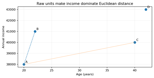
Figure 10.1 — In raw units, the income axis dominates the geometry of the dataset.
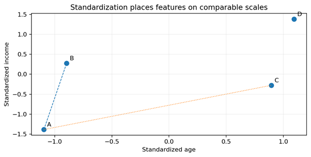
Figure 10.2 — After standardization, age and income contribute on comparable scales.
PYTHON • EXAMPLE 10.1 import numpy as np |
Raw distance is governed mainly by income; standardized distance reflects both variables.
Gradient-based optimization
Logistic regression, linear regression trained by gradient methods, support vector machines, and neural networks minimize a loss function iteratively. When features have very different scales, the loss surface can become elongated: gradients are steep in one direction and shallow in another. Optimization may zigzag, require smaller learning rates, or converge slowly. Scaling creates a better-conditioned optimization problem.
NOTE Scaling does not guarantee a better final model For convex models solved accurately, scaling may mainly improve convergence and coefficient interpretation rather than the best achievable predictive score. For iterative solvers, neural networks, and limited optimization budgets, the practical effect can be substantial. |
Regularization
Regularized linear models penalize coefficient magnitude. Without scaling, a feature measured in large units can use a small coefficient, whereas an equivalent feature measured in small units may require a large coefficient. The penalty then treats them unequally. Standardization makes the penalty more comparable across features.
Objective = data loss + λ Σⱼ |βⱼ|ᵖ For L1 regularization p = 1; for L2 regularization p = 2. Scaling changes how coefficient magnitude relates to feature influence. |
Numerical stability
Very large or very small values can produce poorly conditioned matrices, overflow in exponentials, loss of floating-point precision, or unstable matrix inversion. Scaling reduces these risks. It is especially useful when polynomial features or interactions create values much larger than the original measurements.
PYTHON • EXAMPLE 10.2 import pandas as pd |
An initial range audit reveals variables whose numerical magnitudes differ by several orders.
Scaling is not a substitute for data understanding
- Scaling does not repair incorrect units, impossible values, or data-entry errors.
- Scaling does not make an identifier meaningful or remove target leakage.
- Scaling does not automatically make a skewed distribution symmetric.
- Scaling does not eliminate outliers; some methods can make their influence more visible.
- Scaling must be selected according to the model, distribution, and deployment requirements.
10.2 Standardization
Standardization subtracts the training-set mean and divides by the training-set standard deviation. The transformed feature is expressed in standard-deviation units. In scikit-learn, StandardScaler uses the population standard deviation with divisor n, which is appropriate for transformation even though descriptive statistics often report the sample standard deviation with divisor n − 1.
z = (x − μ) / σ μ is the training mean and σ is the training standard deviation for one feature. |
Mean-centered features
If a feature is transformed with the same mean used during fitting, its training-set mean becomes approximately zero. A value below the mean is negative; a value above the mean is positive. The transformed origin represents the average training observation for that feature.
Unit variance
The transformed training feature has variance approximately one. A standardized value of +2 indicates that the observation is roughly two training standard deviations above the mean. This interpretation is useful only when the mean and standard deviation are informative summaries; extreme outliers can distort both.
PYTHON • EXAMPLE 10.3 import pandas as pd |
Fit learns one mean and one scale per column; transform applies the stored statistics.
Appropriate use cases
- Logistic regression and linear models, especially with L1 or L2 regularization.
- K-nearest neighbors and other distance-based procedures.
- Support vector machines with linear, polynomial, or radial-basis-function kernels.
- Principal component analysis and many dimensionality-reduction methods.
- Neural networks and models trained with gradient descent.
- Numerical features that are roughly symmetric or whose mean and variance are meaningful.
Fitting only on the training set
The validation and test sets must not contribute to the learned mean or standard deviation. Otherwise, information about their distributions influences the training process. The safe sequence is split, fit the scaler on training data, transform training data, and transform held-out data with the same fitted scaler.
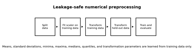
Figure 10.3 — Leakage-safe order for numerical preprocessing.
PYTHON • EXAMPLE 10.4 from sklearn.model_selection import train_test_split |
The test data is transformed with training statistics and remains independent of fitting.
Standardization inside a pipeline
A pipeline is the preferred implementation because cross-validation then refits the scaler separately inside every training fold. It also guarantees that prediction uses exactly the transformation fitted with the model.
PYTHON • EXAMPLE 10.5 from sklearn.pipeline import Pipeline |
One fitted object now contains both numerical preprocessing and the classifier.
Sensitivity to outliers
The mean and standard deviation are not robust statistics. A single extreme value can shift the mean and inflate the standard deviation, compressing most observations into a narrow interval. Standardization is therefore not automatically appropriate for heavy-tailed variables or datasets with severe measurement errors.
Situation | Interpretation | Recommended response |
|---|---|---|
| Rare but valid high values | The tail is part of the population. | Consider log, power, or robust scaling; retain semantic information. |
| Measurement error | The value is not trustworthy. | Correct, remove, or mark the error before scaling. |
| Heavy-tailed financial feature | Mean and standard deviation may be unstable. | Compare RobustScaler and a log/power transformation. |
| Approximately normal measurement | Mean and standard deviation are meaningful. | StandardScaler is a natural baseline. |
PYTHON • EXAMPLE 10.6 import numpy as np |
The extreme value inflates the standard deviation and compresses the central observations.
Inverse transformation
Some workflows need predictions or thresholds expressed in original units. Scalers provide inverse_transform to reconstruct the original scale, subject to floating-point precision. This is particularly useful when the target itself has been transformed for regression.
PYTHON • EXAMPLE 10.7 restored = scaler.inverse_transform(X_train_scaled) |
Inverse transformation should approximately recover the original numerical values.
10.3 Min-max normalization
Min-max normalization maps the training minimum to the lower bound and the training maximum to the upper bound. The default scikit-learn interval is [0, 1], but another fixed interval can be selected. Unlike standardization, min-max scaling does not center the feature or normalize its variance.
x′ = (x − x_min) / (x_max − x_min) For the default [0, 1] range. The minimum and maximum are learned from training data. |
Rescaling to a fixed interval
A fixed interval can be useful when an algorithm or application expects bounded inputs. Neural-network input layers often benefit from comparable bounded ranges, particularly when activation functions saturate. Image pixels are commonly divided by 255 when their valid range is known to be 0–255.
PYTHON • EXAMPLE 10.8 import pandas as pd |
MinMaxScaler records one minimum and maximum for each training feature.
Values outside the training range
A future value greater than the training maximum normally transforms above 1; a value below the training minimum transforms below 0. This behavior is mathematically consistent and can signal distribution shift. The optional clip=True parameter limits transformed values to the requested interval, but clipping hides how far an observation lies outside the historical range.
PYTHON • EXAMPLE 10.9 from sklearn.preprocessing import MinMaxScaler |
Clipping protects downstream ranges but removes information about the magnitude of drift.
Sensitivity to extreme values
The minimum and maximum are determined by the most extreme observations. One outlier can stretch the interval and compress the remaining data near zero. Min-max scaling is therefore suitable when valid bounds are stable and outliers are controlled, but risky for open-ended heavy-tailed variables.
CAUTION A fixed range is not the same as a known physical range Fitting MinMaxScaler to the observed sample uses sample extrema, not necessarily the true physical bounds. For variables with known limits, a domain-defined transformation may be more stable than estimating bounds from a small sample. |
Appropriate use cases
- Inputs with stable, meaningful lower and upper bounds.
- Image pixels or sensor channels with known measurement ranges.
- Neural networks when bounded input scales are helpful.
- K-nearest neighbors or support vector machines when outliers are limited.
- Applications that require all transformed values to share a common interval.
PYTHON • EXAMPLE 10.10 from sklearn.pipeline import make_pipeline |
The scaler and distance-based classifier are trained as one leakage-safe workflow.
10.4 Robust scaling
Robust scaling replaces the mean with the median and the standard deviation with the interquartile range. The median represents the central observation, and the interquartile range covers the middle 50% of values. These statistics are less influenced by a small number of extreme observations.
x_robust = (x − median) / IQR IQR = Q₃ − Q₁, where Q₁ and Q₃ are the 25th and 75th percentiles of the training feature. |
Median and interquartile range
After transformation, the training median is approximately zero. The distance between the first and third quartiles is approximately one when the default quantile range is used. Unlike standardization, robust scaling does not imply unit variance and does not make the distribution normal.
PYTHON • EXAMPLE 10.11 import numpy as np |
The central values remain well separated even though one extreme value is present.
Resistance to outliers
RobustScaler reduces the influence of extreme values on the learned center and scale, but it does not remove or cap those values. An extreme observation may still transform to a very large number. Robust scaling should therefore be combined with domain validation and, when justified, an explicit capping or transformation policy.
Configuring the quantile range
The default quantile range is (25, 75). A wider range such as (10, 90) uses more of the distribution, whereas a narrower range focuses more strongly on its centre. Changing this parameter alters the resulting scale and should be treated as a hyperparameter or documented design choice.
PYTHON • EXAMPLE 10.12 from sklearn.preprocessing import RobustScaler |
A quantile range must be selected consistently and fitted only on training data.
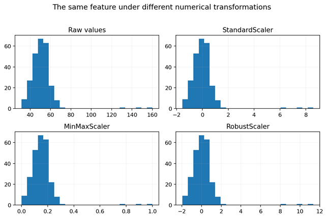
Figure 10.4 — Standard, min-max, and robust scaling react differently to extreme values.
When robust scaling is appropriate
- Financial amounts with long tails and legitimate high-value observations.
- Sensor data with occasional spikes that should not determine the common scale.
- Features whose median and quartiles are more stable than their mean and standard deviation.
- Linear, distance-based, or kernel models that require comparable scales but face moderate outliers.
When robust scaling is not enough
- The outliers are measurement errors requiring correction or removal.
- The distribution spans several orders of magnitude and a log or power transformation is more meaningful.
- The variable has known physical limits that should be encoded directly.
- The feature is multimodal because it combines distinct populations that should be modeled separately.
10.5 Transforming skewed variables
Scaling modifies location and spread, but it usually preserves the overall shape of a distribution. A strongly right-skewed variable remains right-skewed after standardization or min-max scaling. Shape transformations compress or expand parts of the range to reduce skewness, stabilize variance, improve linear relationships, and reduce the influence of very large values.
Logarithmic transformation
The natural logarithm compresses large positive values more strongly than small values. It is appropriate when effects are multiplicative, ratios are meaningful, or a variable spans several orders of magnitude. The function log1p(x) computes log(1 + x), handles zero naturally, and is numerically stable for small values.
x_log = log(1 + x) Valid for x > −1. For nonnegative counts and monetary values, log1p is often convenient. |
PYTHON • EXAMPLE 10.13 import numpy as np |
Large multiplicative differences become smaller additive differences after the logarithm.
Square-root transformation
The square root is milder than the logarithm and is commonly used for nonnegative counts. It can reduce moderate right skew while preserving zero. The transformation is not appropriate for negative values unless a justified shift is applied.
PYTHON • EXAMPLE 10.14 counts = pd.Series([0, 1, 2, 4, 9, 25, 100], name="incident_count") |
Square-root transformation is often useful for count-like features with moderate skew.
Power transformation
Power transformations learn an exponent that makes a distribution more Gaussian-like. Box–Cox requires strictly positive values. Yeo–Johnson supports zero and negative values and is therefore more broadly applicable. scikit-learn can optionally standardize the transformed output.
Method | Allowed values | Learned parameter | Typical use |
|---|---|---|---|
| Box–Cox | Strictly positive | One λ per feature | Positive continuous features. |
| Yeo–Johnson | Negative, zero, and positive | One λ per feature | General continuous numerical features. |
| Manual log1p | Values greater than −1 | No learned exponent | Known multiplicative relationship or long right tail. |
PYTHON • EXAMPLE 10.15 from sklearn.preprocessing import PowerTransformer |
Yeo–Johnson learns transformation parameters from training data and reuses them on held-out data.
Quantile transformation
A quantile transformer maps values according to their empirical cumulative distribution. It can produce an approximately uniform or normal marginal distribution and strongly reduce the influence of extreme values. Because it is nonlinear and rank-based, it can alter distances and linear relationships substantially. It may also map unseen extremes to the bounds learned from training data.
PYTHON • EXAMPLE 10.16 from sklearn.preprocessing import QuantileTransformer |
Quantile transformation is powerful but should be validated carefully because it changes feature geometry nonlinearly.
Selecting a transformation
Observed pattern | Candidate transformation | Reason to test it |
|---|---|---|
| Positive values spanning orders of magnitude | log or log1p | Compresses multiplicative scale and long right tail. |
| Nonnegative count with moderate skew | square root | Milder compression and preserves zero. |
| Continuous values including zeros or negatives | Yeo–Johnson | Learns a flexible monotonic power transformation. |
| Strictly positive continuous feature | Box–Cox | Learns a power transformation under positivity. |
| Severe tails or desired normal marginal | QuantileTransformer | Uses empirical ranks and limits tail influence. |
| Already symmetric and stable | No shape transformation | Avoid unnecessary complexity. |
Preserving interpretability
A transformation changes the meaning of a one-unit difference. Coefficients then describe the relationship with the transformed feature, not the raw feature. Domain users may find a coefficient for log income harder to interpret. The model documentation should record the exact transformation, fitted parameters, valid input domain, and inverse interpretation when possible.
GOOD PRACTICE Compare transformed and untransformed baselines Apply a shape transformation because it improves validation performance, residual behavior, numerical stability, or domain consistency—not merely because a histogram looks more symmetric. |
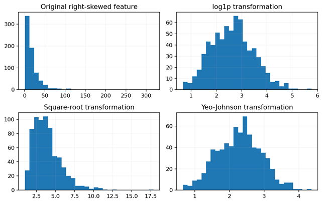
Figure 10.5 — Common transformations reduce right skew to different degrees.
PYTHON • EXAMPLE 10.17 from sklearn.compose import ColumnTransformer |
Different numerical columns can receive different transformations in one reproducible pipeline.
10.6 Models requiring scaling
Scale sensitivity depends on the mathematical operations used by the model. Algorithms based on distances, dot products, gradients, covariance, or coefficient penalties are usually sensitive. Tree-based algorithms compare one feature with a threshold at a time, so monotonic rescaling generally leaves their split ordering unchanged.
Models for which scaling is usually important
Model family | Why scale matters | Common choice |
|---|---|---|
| Logistic regression | Optimization and regularization depend on feature magnitude. | StandardScaler; RobustScaler for outliers. |
| Ridge, Lasso, Elastic Net | Coefficient penalties must treat features comparably. | StandardScaler. |
| K-nearest neighbors | Distance is directly computed from feature differences. | StandardScaler or MinMaxScaler. |
| Support vector machines | Margins, kernels, C, and gamma depend on geometry. | StandardScaler is a strong default. |
| Neural networks | Gradient conditioning and activation ranges affect learning. | StandardScaler or bounded scaling, depending on architecture. |
| PCA and covariance methods | High-variance raw features can dominate components. | StandardScaler when units differ. |
Models for which scaling is generally less important
Model family | Why scale matters less | Important qualification |
|---|---|---|
| Decision trees | Split ordering is unchanged by monotonic scaling. | Outliers and skew can still affect data quality and interpretation. |
| Random forests | Each tree uses threshold splits on individual features. | Scaling normally does not change predictions materially. |
| Gradient-boosted trees | Tree learners remain based on ordered thresholds. | Histogram binning and numerical precision may create small implementation differences. |
| Rule-based models | Rules compare explicit values or categories. | Thresholds must still be expressed in correct units. |
Scale sensitivity is not binary
Some algorithms are indirectly affected. Naive Bayes estimates per-feature distributions and does not usually require scaling, but transformations may improve distribution assumptions. Linear discriminant analysis can be sensitive to covariance conditioning even though the theoretical classifier is invariant to some rescalings. The correct approach is to understand the algorithm and validate the complete pipeline.
PYTHON • EXAMPLE 10.18 from sklearn.model_selection import cross_val_score, StratifiedKFold |
Each cross-validation fold fits its own scaler because preprocessing is inside the pipeline.
Sparse matrices and centering
One-hot encoded features are often stored in sparse matrices. Subtracting the mean makes almost every zero nonzero and destroys sparsity. StandardScaler(with_mean=False) scales sparse features without centering. MaxAbsScaler is another option because it preserves zeros and scales by maximum absolute value.
PYTHON • EXAMPLE 10.19 from sklearn.preprocessing import StandardScaler, MaxAbsScaler |
Never center a large sparse matrix unless densification is intentional and memory-safe.
Target preprocessing in regression
A highly skewed continuous target can also be transformed, but target transformation is conceptually different from feature preprocessing. TransformedTargetRegressor applies a transformation during fitting and automatically converts predictions back to the original target scale.
PYTHON • EXAMPLE 10.20 import numpy as np |
The regressor learns the log-transformed target while users receive predictions in original units.
Decision guide
Question | Yes | No |
|---|---|---|
| Does the model use distances, dot products, gradients, or coefficient penalties? | Begin with a scaling pipeline. | Scaling may be optional; check the algorithm. |
| Are strong outliers legitimate and retained? | Compare robust scaling and shape transformations. | Standard or min-max scaling may be adequate. |
| Does the feature span orders of magnitude? | Consider log or power transformation before scaling. | A simple scaler may suffice. |
| Are physical bounds stable and meaningful? | Domain scaling or min-max may be suitable. | Avoid assuming sample extrema are fixed bounds. |
| Is the feature matrix sparse? | Use a sparse-safe scaler without centering. | Standard centering is normally safe. |
Practical lab — Comparing models with and without scaling
In this lab, students build a classification dataset whose features have deliberately different numerical scales. They compare no scaling, standardization, min-max normalization, and robust scaling across algorithms with different scale sensitivities. All transformations are embedded in pipelines so that cross-validation remains leakage-safe.
Learning goals
- Measure how feature scale changes validation performance for logistic regression, KNN, and SVM.
- Verify that a random forest is comparatively insensitive to monotonic numerical scaling.
- Compare mean performance and fold-to-fold variability.
- Inspect transformed distributions and learned scaler statistics.
- Write a defensible recommendation rather than declaring one scaler universally best.
Lab setup and evaluation protocol
Element | Configuration |
|---|---|
| Dataset | 1,500 synthetic observations, six numerical features, and a binary target. |
| Preprocessing candidates | No scaling, StandardScaler, MinMaxScaler, and RobustScaler. |
| Models | Logistic regression, KNN, RBF SVM, and random forest. |
| Validation | Five-fold stratified cross-validation with shuffling and random_state=42. |
| Primary metrics | ROC AUC, F1-score, fold-to-fold standard deviation, and fitting time. |
| Fair-comparison rule | All configurations use the same folds, metrics, and preprocessing pipeline structure. |
Step 1 — Create the dataset
PYTHON • LAB 10.1 import numpy as np |
The features contain useful signal but their numerical scales differ greatly.
Step 2 — Define preprocessing alternatives
PYTHON • LAB 10.2 from sklearn.preprocessing import StandardScaler, MinMaxScaler, RobustScaler |
Each candidate will be inserted into a pipeline and fitted independently in every fold.
Step 3 — Define candidate algorithms
PYTHON • LAB 10.3 from sklearn.linear_model import LogisticRegression |
The first three algorithms are scale-sensitive; the random forest is the comparison model.
Step 4 — Evaluate every combination
PYTHON • LAB 10.4A from sklearn.model_selection import StratifiedKFold, cross_validate |
Every scaler–model pair is evaluated on the same stratified folds.
PYTHON • LAB 10.4B records.append({ |
Use the same folds and metrics for every configuration to ensure a fair comparison.
Step 5 — Visualize the comparison
PYTHON • LAB 10.5 import matplotlib.pyplot as plt |
A bar chart should show large scaling effects for some models and minimal effects for the forest.
Step 6 — Inspect fitted scaler statistics
PYTHON • LAB 10.6 from sklearn.pipeline import make_pipeline |
Fitted preprocessing parameters are part of the final model artifact and should be documented.
Step 7 — Add a skew-aware alternative
PYTHON • LAB 10.7 from sklearn.compose import ColumnTransformer |
The experiment tests whether shape correction adds value beyond simple scaling.
Required lab report
- State the dataset dimensions, class proportions, and raw feature ranges.
- Provide a results table containing mean ROC AUC, standard deviation, mean F1-score, and fit time.
- For each algorithm, identify the best preprocessing method and quantify its improvement over no scaling.
- Explain why KNN and SVM are expected to react more strongly than random forests.
- Discuss whether standardization, min-max normalization, robust scaling, or log-plus-standardization is the most defensible final choice.
- Document leakage prevention: preprocessing must be fitted inside each cross-validation training fold.
- State at least two limitations of the experiment and one next step.
Expected interpretation
EXPECTED OUTCOME There is no universally best scaler Students should normally observe that scale-sensitive algorithms benefit from suitable preprocessing, while random-forest performance changes little. The exact ranking of StandardScaler, MinMaxScaler, RobustScaler, and the skew-aware pipeline can vary with the generated sample and evaluation metric. The report must explain the pattern rather than merely list the highest score. |
Common mistakes and how to avoid them
Mistake | Why it is wrong | Correct practice |
|---|---|---|
| Fit the scaler before splitting | Held-out statistics influence training. | Split first or place preprocessing in a pipeline. |
| Fit separately on test data | Training and test are expressed in different coordinate systems. | Transform test data with the fitted training scaler. |
| Scale identifiers | An arbitrary ID becomes a numerical signal. | Remove IDs or use them only for grouping and traceability. |
| Assume scaling removes outliers | Most scalers only change coordinates. | Diagnose, validate, cap, transform, or use robust methods. |
| Apply log to negative values without checking | The transformation is undefined. | Validate domain or use Yeo–Johnson. |
| Use min-max because values “must be 0–1” | Future data may exceed the observed range. | Define how drift and clipping will be handled. |
| Center a sparse matrix | The matrix may densify and exhaust memory. | Use with_mean=False or MaxAbsScaler. |
| Scale tree models automatically | It adds complexity with little benefit. | Keep it only if the shared pipeline or other transforms justify it. |
| Select a scaler using test performance | The test set becomes part of model selection. | Select through validation or cross-validation. |
Knowledge check
1. A KNN model uses age (18–90) and income (20,000–400,000). What is the primary risk?
2. Why does StandardScaler usually belong inside a cross-validation pipeline?
3. Does standardization make a skewed feature normally distributed?
4. Which method is less influenced by a few extreme values: StandardScaler or RobustScaler?
5. Can MinMaxScaler produce values greater than 1?
6. Which power method accepts zero and negative values?
7. Why do regularized linear models need comparable feature scales?
8. Why do decision trees usually not require scaling?
Answers
1. Income will dominate Euclidean distance unless features are rescaled.
2. Its mean and standard deviation must be learned independently from each training fold.
3. No. It changes location and spread, not generally distribution shape.
4. RobustScaler, because it uses the median and interquartile range.
5. Yes, when future values exceed the training maximum unless clipping is enabled.
6. Yeo–Johnson.
7. Otherwise coefficient penalties treat features differently because of arbitrary units.
8. Monotonic scaling preserves feature ordering and therefore candidate threshold partitions.
Chapter summary
- Scaling changes the numerical representation of features but does not add information or repair data errors.
- Standardization creates zero-centred, unit-variance training features and is a strong default for many linear, distance-based, kernel, and gradient-based models.
- Min-max normalization maps the observed training range to a fixed interval but is highly sensitive to extrema and future range violations.
- Robust scaling uses the median and interquartile range, reducing the influence of a small number of extreme observations.
- Logarithmic, square-root, power, and quantile transformations address distribution shape rather than only feature scale.
- Tree-based models usually need little or no numerical scaling because monotonic transformations preserve feature ordering.
- All learned preprocessing must be fitted on training data only; pipelines are the safest implementation for cross-validation and deployment.
- The correct transformation is selected through domain reasoning, distribution analysis, and validation—not by a universal rule.
Key terms
Term | Meaning |
|---|---|
| Scaling | Changing the numerical location or spread of a feature. |
| Standardization | Subtracting the mean and dividing by the standard deviation. |
| Normalization | Often used for mapping values to a fixed interval or scaling vectors to unit norm; context must be stated. |
| Robust scaling | Centering by the median and scaling by an interquantile range. |
| Skewness | Asymmetry of a distribution around its centre. |
| Power transformation | A monotonic transformation controlled by a learned exponent. |
| Quantile transformation | A rank-based mapping to a target marginal distribution. |
| Numerical conditioning | How sensitively a numerical computation responds to small changes or finite precision. |
| Data leakage | Use of information outside the permitted training data during fitting or model selection. |
| Pipeline | An ordered object that fits preprocessing and a model as one reproducible workflow. |
Practical checklist
- Confirm units, valid ranges, and missing-value handling before scaling.
- Inspect distribution shape and outliers for every numerical feature.
- Choose transformations column by column when feature characteristics differ.
- Split data before fitting any data-dependent transformation.
- Use Pipeline and ColumnTransformer for cross-validation and production inference.
- Compare preprocessing alternatives using identical validation folds and metrics.
- Record fitted transformation type, parameters, feature order, and library versions.
- Monitor future values for range violations and distribution drift.
FINAL OUTCOME What students should now be able to do Students can diagnose scale and skew problems, choose and implement an appropriate numerical transformation, prevent preprocessing leakage, compare alternatives fairly, and explain why the selected method is suitable for both the algorithm and the deployment data. |