Chapter 3 — The Complete Supervised Learning Workflow
Chapter overview
A successful supervised learning project is not a single call to a training function. It is a controlled sequence of decisions about the problem, data, validation strategy, candidate models, evaluation criteria, interpretation, delivery, and monitoring. A weakness in any one stage can invalidate the final result, even when the selected algorithm is technically sophisticated.
This chapter presents a complete workflow that can be reused for classification and regression. The emphasis is on experimental discipline: the test set remains untouched, transformations are learned only from training data, candidate models are compared under the same conditions, and every important decision is recorded. A synthetic customer-churn example is used throughout the Python sections so that the complete notebook can be executed without downloading external data.
KEY IDEA The workflow is iterative, not merely linear The numbered sequence provides a clear first pass, but real projects often move backward. Error analysis can reveal a data-quality problem, monitoring can trigger retraining, and feature interpretation can expose leakage. Iteration is valuable when each change is documented and re-evaluated under the same validation protocol. |
Learning objectives
- Describe the fifteen main stages of an end-to-end supervised learning project.
- Distinguish the roles of training, validation, cross-validation, and testing data.
- Construct a leakage-resistant preprocessing and modeling pipeline.
- Establish meaningful baselines and compare candidate algorithms fairly.
- Tune hyperparameters without using the test set.
- Record configurations, random seeds, transformations, metrics, and artifacts for reproducibility.
- Recognize common workflow mistakes and replace them with defensible practices.
- Design a workflow diagram for a new supervised learning project.
Running example and notebook conventions
The code examples model customer churn as a binary classification problem. Each row represents one customer at a defined prediction date. The target equals 1 when that customer leaves during the following observation window and 0 otherwise. Numerical and categorical features are included, and a small amount of missing data is introduced to demonstrate realistic preprocessing.
Element | Running example |
|---|---|
| Unit of observation | One customer at the prediction date |
| Target | churn: 1 = leaves during the next period; 0 = remains |
| Numerical features | tenure_months, monthly_charge, support_tickets, late_payments, usage_score |
| Categorical features | contract_type and region |
| Primary metric | ROC AUC for model comparison; recall and precision for operational review |
| Final deliverable | A serialized preprocessing-and-model pipeline plus evaluation report |
Chapter map
Section | Purpose |
|---|---|
| 3.1 Main workflow | Develop the complete project from problem definition to monitoring. |
| 3.2 Experimental discipline | Protect the validity, fairness, and reproducibility of experiments. |
| 3.3 Common mistakes | Identify workflow failures that create optimistic or unusable results. |
| Practical activity | Create and justify a workflow diagram for a supervised learning project. |
3.1 Main Workflow
The complete workflow contains fifteen connected stages. Some stages create technical artifacts, such as a fitted pipeline or a metric report. Others create decision artifacts, such as a target definition, data contract, risk statement, or deployment threshold. A professional workflow treats both categories as essential.
Governing principles
Principle | Meaning |
|---|---|
| Separation of roles | Training learns parameters, validation supports decisions, and testing estimates final generalization. |
| Whole-pipeline evaluation | Preprocessing and the estimator are evaluated together under the same data boundaries. |
| Lifecycle ownership | The project includes delivery, monitoring, retraining criteria, and retirement—not only model fitting. |
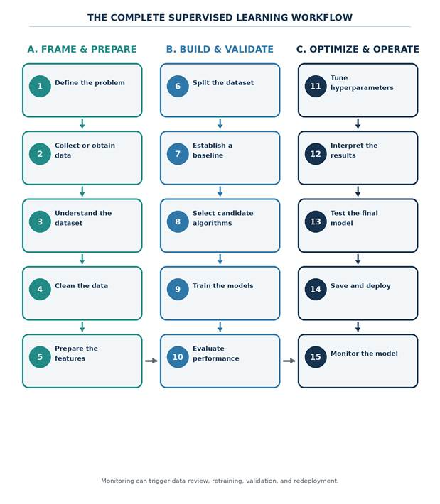
Figure 3.1 — The fifteen-stage supervised learning workflow.
Workflow deliverables at a glance
Stage | Core question | Main artifact |
|---|---|---|
| 1. Define the problem | What decision or prediction is required? | Problem statement and success criteria |
| 2. Obtain data | Which historical examples are available and lawful to use? | Dataset inventory and provenance record |
| 3. Understand data | What does each row and column mean? | Data dictionary and exploratory report |
| 4. Clean data | Which quality problems must be corrected? | Cleaning rules and quality log |
| 5. Prepare features | How will raw variables become model inputs? | Feature specification and preprocessing plan |
| 6. Split data | How will future or unseen performance be simulated? | Train/validation/test split protocol |
| 7. Establish baseline | What simple result must the model exceed? | Dummy or rule-based baseline |
| 8. Select algorithms | Which model families suit the task and constraints? | Candidate model shortlist |
| 9. Train models | How are identical training conditions applied? | Fitted candidate pipelines |
| 10. Evaluate | Which model generalizes best under the chosen criteria? | Cross-validation comparison report |
| 11. Tune | Which hyperparameters improve the selected candidates? | Search results and chosen configuration |
| 12. Interpret | Why does the model behave as observed? | Global and local interpretation report |
| 13. Final test | What is the unbiased final estimate? | Locked test-set evaluation |
| 14. Save/deploy | How will predictions be delivered safely? | Versioned model artifact and interface |
| 15. Monitor | How will drift and degradation be detected? | Monitoring and retraining plan |
3.1.1 Define the Problem
Problem definition determines every later choice. The team must state the predicted outcome, the unit of observation, the prediction horizon, the moment at which features are available, the intended user, and the action that follows a prediction. Without these details, a technically accurate model may answer the wrong question.
For customer churn, “predict churn” is incomplete. A usable formulation might be: “At the end of each month, estimate the probability that each active customer will cancel during the next 30 days, using information available before the scoring date, so that the retention team can prioritize a limited number of interventions.”
Problem component | Question to answer | Churn example |
|---|---|---|
| Unit of observation | What does one row represent? | One active customer at month-end |
| Target | What outcome is predicted? | Cancellation within the next 30 days |
| Prediction time | When is the model executed? | Last day of each month |
| Feature cutoff | What information is allowed? | Data recorded no later than month-end |
| User and action | Who acts on the result? | Retention team contacts selected customers |
| Error costs | Which mistakes matter? | False negatives lose customers; false positives consume capacity |
| Success criterion | What level of value is required? | Improved recall at a feasible contact volume |
GOOD PRACTICE Define the target before inspecting model scores Changing the target from cancellation within 30 days to cancellation within 90 days creates a different dataset, operational process, and evaluation problem. The target definition must be versioned like code. |
3.1.2 Collect or Obtain Data
Data may come from databases, files, APIs, surveys, sensors, experiments, logs, or public repositories. Collection is not only a technical task. The project must document provenance, permissions, time coverage, sampling mechanisms, label generation, and known limitations. Historical records reflect the process that produced them; they are not automatically representative of future use.
- Identify authoritative sources and assign an owner to each source.
- Record extraction dates, query versions, filters, and row counts.
- Verify that labels were generated consistently across time and groups.
- Confirm privacy, consent, retention, licensing, and security requirements.
- Preserve an immutable raw snapshot before cleaning or feature construction.
- Check whether important populations or rare events are underrepresented.
PYTHON • EXAMPLE 3.1 — CREATE A REPRODUCIBLE DEMONSTRATION DATASET import numpy as np Run this cell once at the start of the notebook. The same random seed recreates the same demonstration dataset. |
3.1.3 Understand the Dataset
Data understanding combines semantic review and exploratory analysis. Semantic review asks what each field means, how it was measured, when it became available, and whether its meaning changed. Exploratory analysis examines distributions, missingness, duplicates, target prevalence, relationships, outliers, and unexpected values.
A data dictionary should distinguish identifiers, features, targets, timestamps, grouping variables, and fields excluded from modeling. Identifiers such as customer_id are useful for joining predictions back to business systems but are usually not predictive inputs. Timestamps may define split boundaries even when they are not model features.
PYTHON • EXAMPLE 3.2 — PRODUCE AN INITIAL DATA AUDIT def audit_dataframe(data: pd.DataFrame, target: str) -> pd.DataFrame: The audit is a starting point, not a substitute for a domain expert’s review of definitions and collection processes. |
CAUTION Unexpectedly strong predictors require investigation A column that almost perfectly predicts the target may be genuinely informative, but it may also encode an event that occurs after the outcome, a manually assigned status derived from the label, or a duplicated identifier. Treat suspicious performance as a data question before celebrating it as a modeling success. |
3.1.4 Clean the Data
Cleaning removes or corrects defects that prevent valid analysis. Typical tasks include resolving duplicate entities, standardizing categories, converting units, parsing dates, handling impossible values, and deciding how missingness will be treated. Cleaning rules should be explicit and deterministic so that the same logic can later be applied to new data.
Issue | Example | Defensible response |
|---|---|---|
| Missing value | monthly_charge is absent | Investigate cause; impute within the training pipeline and optionally add a missing indicator |
| Invalid range | usage_score = 145 although valid range is 0–100 | Correct from source, set to missing, or reject row according to a documented rule |
| Inconsistent category | Monthly, monthly, MONTHLY | Normalize case and map to one controlled vocabulary |
| Duplicate entity | Same customer and scoring date repeated | Define the authoritative record or aggregation rule |
| Unit inconsistency | Charges recorded in different currencies | Convert using a documented historical or contractual rule |
| Label inconsistency | Cancellation definition changed mid-year | Version the label and reconsider time coverage or stratification |
GOOD PRACTICE Do not hide cleaning decisions in ad hoc notebook cells Cleaning logic should live in reusable functions, SQL transformations, validation rules, or versioned pipelines. A later reader must be able to identify exactly which rows and values were modified. |
3.1.5 Prepare the Features
Feature preparation converts raw fields into numerical representations suitable for candidate algorithms. Numerical features may require imputation, scaling, transformation, or clipping. Categorical features commonly require imputation and one-hot or ordinal encoding. Dates may generate calendar or duration features. Text, images, and signals require specialized representations.
Any transformation that estimates a statistic from data—mean, median, scaling parameters, vocabulary, category frequencies, selected features, or learned embeddings—must be fitted on training data only. A scikit-learn pipeline makes this boundary explicit and applies identical transformations during validation, testing, and deployment.
Feature type | Typical preparation | Important risk |
|---|---|---|
| Numerical | Median imputation; optional standardization or log transform | Using full-dataset mean or standard deviation |
| Nominal categorical | Most-frequent imputation and one-hot encoding | Unseen categories at prediction time |
| Ordinal | Ordered encoding based on domain meaning | Inventing an order that does not exist |
| Date/time | Durations, recency, seasonality, day-of-week | Using future timestamps or post-outcome information |
| Text | TF–IDF, embeddings, language-specific processing | Vocabulary fitted before splitting or privacy leakage |
| Image/signal | Normalization, windows, descriptors, learned representations | Related samples from one entity split across datasets |
3.1.6 Split the Dataset
The split strategy approximates how the model will encounter future unseen cases. Random splitting can be appropriate for independent and identically distributed observations. Stratified splitting preserves class proportions. Grouped splitting keeps all records from the same customer, patient, device, or subject together. Time-based splitting trains on earlier periods and evaluates on later periods.
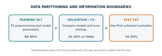
Figure 3.2 — Training, validation, and test data serve different purposes.
KEY IDEA The test set is a sealed final exam Do not inspect its metrics repeatedly, use it to choose features, select a threshold, or decide between algorithms. Every such use turns the test set into another validation set and makes the reported performance optimistic. |
PYTHON • EXAMPLE 3.3 — SPLIT FIRST AND CONSTRUCT A PREPROCESSING PIPELINE from sklearn.compose import ColumnTransformer No imputer, scaler, or encoder is fitted yet. They will learn statistics only inside each training fold. |
3.1.7 Establish a Baseline
A baseline establishes the minimum performance that a trained model must exceed. For classification, a DummyClassifier can always predict the majority class or sample according to class proportions. For regression, a DummyRegressor can always predict the training mean or median. A domain rule may provide a stronger operational baseline.
A baseline can expose a misleading metric. In a dataset with 98% negative cases, a classifier that predicts the negative class for everyone obtains 98% accuracy but detects none of the positive cases. Baselines should therefore be evaluated with metrics aligned to the project objective.
Baseline | Purpose | Interpretation |
|---|---|---|
| Majority-class classifier | Checks whether a model beats the most frequent label | Useful accuracy floor, but may have zero minority recall |
| Stratified random classifier | Checks whether ranking or probability metrics beat chance | Expected ROC AUC is near 0.5 |
| Mean/median regressor | Provides a no-feature regression reference | Candidate models must reduce prediction error |
| Domain rule | Represents current practice or policy | Most important baseline when replacing an existing process |
3.1.8 Select Candidate Algorithms
Candidate selection should cover several model families while respecting data size, latency, interpretability, probability requirements, and maintenance constraints. A compact, diverse shortlist is more informative than an indiscriminate catalogue of algorithms.
Model family | Strengths | Limitations / requirements |
|---|---|---|
| Logistic regression | Fast, interpretable, calibrated baseline, strong for approximately linear effects | Requires encoding; scaling helps; limited nonlinear interactions |
| Decision tree | Readable rules, nonlinear splits, limited preprocessing | High variance and easy overfitting |
| Random forest | Robust nonlinear baseline, interactions, limited scaling needs | Larger artifact; probabilities may need calibration |
| Gradient boosting | Often excellent on structured tabular data | More tuning; training and interpretation are more complex |
| Support vector machine | Strong decision boundaries on medium-sized datasets | Scaling required; can be expensive; probabilities are optional |
| K-nearest neighbors | Simple local model and useful teaching tool | Scaling required; slow prediction; sensitive to dimensionality |
GOOD PRACTICE Complexity must earn its place A more complex model is justified only when it provides a reliable improvement large enough to outweigh reduced interpretability, higher latency, tuning effort, maintenance cost, or operational risk. |
3.1.9 Train the Models
Training estimates model parameters from the training data. For fair comparison, all candidates should use the same feature definition, cross-validation folds, scoring metrics, and preprocessing discipline. Each candidate should be represented as one complete pipeline so that preprocessing is refitted independently inside every training fold.
PYTHON • EXAMPLE 3.4 — COMPARE BASELINES AND CANDIDATE PIPELINES from sklearn.dummy import DummyClassifier Cross-validation refits the preprocessing steps and estimator inside each fold, preventing statistics from leaking from validation folds into training. |
3.1.10 Evaluate Performance
Evaluation asks whether the model generalizes, whether its errors are acceptable, and whether performance is stable across folds, time periods, and relevant subgroups. A single average score is insufficient. Report variability, confusion-matrix quantities, probability quality when needed, computation time, and failure patterns.
Question | Classification evidence | Regression evidence |
|---|---|---|
| Does the model discriminate or rank well? | ROC AUC; precision-recall AUC | Correlation and explained variation may provide context |
| How large are the errors? | False-positive and false-negative counts or rates | MAE, RMSE, quantile errors |
| Are predictions operationally useful? | Precision/recall at chosen threshold or capacity | Error within acceptable tolerance |
| Are probabilities trustworthy? | Log loss, Brier score, calibration curve | Prediction intervals or uncertainty estimates |
| Is performance stable? | Fold, time, source, and subgroup comparisons | Residuals and slice-level error comparisons |
KEY IDEA Choose the primary metric before comparing models The primary metric encodes the project objective. Secondary metrics help explain trade-offs, but selecting whichever metric looks best after training encourages result shopping and weakens the experiment. |
3.1.11 Tune Hyperparameters
Hyperparameters control model capacity, regularization, learning behavior, and computational trade-offs. They are selected using validation data or cross-validation—not the test set. Search spaces should be motivated by model behavior and available resources. Randomized search is often more efficient than an exhaustive grid when many parameters are considered.
Tuning should follow an initial comparison. Spending a large search budget on every candidate can waste resources and increase the chance of overfitting the validation procedure. Usually one or two promising model families are tuned more carefully.
PYTHON • EXAMPLE 3.5 — TUNE A CANDIDATE WITHOUT TOUCHING THE TEST SET from scipy.stats import randint, loguniform RandomizedSearchCV selects settings using only the training portion and refits the best complete pipeline on all training rows. |
3.1.12 Interpret the Results
Interpretation examines what the model learned, why individual predictions occur, and whether behavior is plausible. Linear coefficients, tree-based importance, permutation importance, partial dependence, and SHAP values answer different questions and have different limitations. Interpretation should be combined with domain review and error analysis.
- Global interpretation: Which features influence predictions across the dataset?
- Local interpretation: Which feature values contributed to one specific prediction?
- Error analysis: Which types of observations produce false positives, false negatives, or large residuals?
- Sensitivity analysis: How do predictions change when a feature is perturbed within a realistic range?
- Sanity checks: Does the model rely on identifiers, post-outcome variables, proxies, or implausible relationships?
CAUTION Importance is not causality A feature can improve prediction because it correlates with the target. This does not establish that changing the feature will change the outcome. Causal claims require a different design and stronger assumptions. |
3.1.13 Test the Final Model
After the model family, preprocessing, hyperparameters, and decision rule have been finalized, the complete pipeline is evaluated once on the untouched test set. This provides the closest available estimate of performance on comparable unseen data. The test report should include the primary metric, important secondary metrics, uncertainty or confidence intervals where possible, and limitations.
PYTHON • EXAMPLE 3.6 — PERFORM THE LOCKED FINAL TEST EVALUATION from sklearn.metrics import ( The decision threshold must also be selected without using the test labels. Freeze it before this cell is executed. |
3.1.14 Save and Deploy the Model
Deployment makes the trained pipeline available to another process. Predictions may be generated in a scheduled batch, through an API, inside a web application, or on an edge device. The serialized artifact should include preprocessing and the estimator together, accompanied by model metadata, an input schema, version information, and tests.
Deployment concern | Required control |
|---|---|
| Input schema | Validate required columns, types, ranges, units, and allowed categories |
| Versioning | Assign versions to code, data snapshot, feature definition, and model artifact |
| Dependency compatibility | Record Python and library versions; rebuild artifacts when necessary |
| Security | Never load untrusted pickle/joblib files; restrict artifact access |
| Latency and capacity | Measure prediction time, memory, batch size, and concurrent load |
| Fallback behavior | Define what happens when input is invalid or the model is unavailable |
| Traceability | Log model version, scoring time, input identifiers, and outputs appropriately |
PYTHON • EXAMPLE 3.7 — SAVE, LOAD, VALIDATE, AND REUSE THE PIPELINE from pathlib import Path Serialization formats such as joblib and pickle can execute code when loaded. Load only artifacts produced and stored by trusted systems. |
3.1.15 Monitor the Model
A deployed model operates in a changing environment. Input distributions can drift, categories can appear or disappear, data pipelines can fail, user behavior can change, and the relationship between features and outcomes can weaken. Monitoring detects these changes early enough to investigate, retrain, recalibrate, or roll back.
Monitoring layer | Examples | Possible response |
|---|---|---|
| Service health | Latency, errors, throughput, memory, missing predictions | Scale service, repair dependency, activate fallback |
| Schema and quality | Missing columns, invalid types, out-of-range values, unseen categories | Reject or quarantine records; repair upstream data |
| Input drift | Changes in feature distributions or category proportions | Investigate source/process change; schedule review |
| Prediction drift | Changes in score, class, confidence, or abstention distribution | Check data shift, threshold, and capacity assumptions |
| Performance | Recall, precision, AUC, MAE, calibration after labels arrive | Recalibrate, retrain, redesign features, or retire model |
| Fairness and slices | Error rates across relevant groups, regions, devices, or time periods | Investigate representation and process differences |
PYTHON • EXAMPLE 3.8 — RECORD SIMPLE PRODUCTION-QUALITY SIGNALS def monitoring_snapshot(batch: pd.DataFrame, probabilities: np.ndarray) -> dict: A production system should compare these signals with reference ranges, attach timestamps and model versions, and alert only when predefined conditions are met. |
KEY IDEA Monitoring closes the lifecycle When labels become available, compare current performance with the validated reference. A retrained model must pass the same validation and test gates before replacing the deployed version. |
3.2 Experimental Discipline
Experimental discipline protects the credibility of results. It separates exploration from final evaluation, makes comparisons fair, and ensures that another person can reconstruct what was done. The goal is not to eliminate iteration but to make every iteration traceable and scientifically defensible.
3.2.1 Keeping the Test Set Untouched
The test set is reserved for one final evaluation after all modeling choices have been fixed. This includes feature inclusion, preprocessing, candidate selection, hyperparameters, calibration method, decision threshold, and metric definitions. Looking at test results during development creates feedback: the team unconsciously adapts decisions to the test cases, and the final estimate becomes optimistic.
Allowed before final testing | Not allowed before final testing |
|---|---|
| Inspect training data and cross-validation results | Use test labels to choose features or algorithms |
| Select a metric and validation strategy | Tune hyperparameters on test performance |
| Choose a threshold using validation predictions | Adjust the threshold after seeing the test confusion matrix |
| Debug code using synthetic or training examples | Repeatedly inspect test errors and revise the model |
| Verify test schema without studying labels | Report the best of many test-set experiments |
CAUTION What if the test set has already been used repeatedly? Treat it as validation data. Create a new final test set from a later time period, a new source, or an independently held-out sample. Clearly document why the original test estimate is no longer unbiased. |
3.2.2 Recording Model Configurations
A result without its configuration is not reproducible. Record algorithm names, hyperparameters, preprocessing choices, feature lists, random seeds, data snapshot identifiers, split rules, metrics, library versions, and output artifacts. Configuration files or structured dictionaries are preferable to scattered constants across notebook cells.
Record | Example |
|---|---|
| Experiment identifier | churn_rf_2026_08_01_001 |
| Data version | warehouse snapshot 2026-07-31; extraction query commit a92f… |
| Split rule | 80/20 stratified random split; random_state=42 |
| Feature version | churn_features_v3; seven input variables |
| Preprocessing | median imputation, standardization, one-hot encoding |
| Estimator | RandomForestClassifier |
| Hyperparameters | n_estimators=514, max_depth=12, min_samples_leaf=6 |
| Primary metric | five-fold stratified CV ROC AUC |
| Artifact paths | model, report, predictions, environment specification |
3.2.3 Controlling Random Seeds
Randomness can enter data splitting, resampling, model initialization, feature subsampling, and hyperparameter search. Fixed seeds make debugging and comparison easier. They do not guarantee identical results across all hardware, parallel execution orders, or library versions, and they do not replace repeated validation. The seed itself should be part of the experiment record.
PYTHON • EXAMPLE 3.9 — CENTRALIZE EXPERIMENT SETTINGS from dataclasses import asdict, dataclass Centralized settings reduce accidental inconsistencies between data splitting, cross-validation, model training, and saved reports. |
3.2.4 Tracking Data Transformations
Every transformation should have a defined input, output, fitted state, and purpose. Pipelines provide an executable record, while feature specifications and data dictionaries provide human-readable context. Track transformations that occur upstream as well as those inside the model pipeline.
Transformation question | Why it matters |
|---|---|
| Was the transformation fitted or rule-based? | Fitted transformations must learn from training data only. |
| What columns and units are expected? | Prevents silent schema or unit mismatches. |
| How are missing and unknown values handled? | Determines whether deployment can process real inputs safely. |
| Does the transformation use time or target information? | Reveals temporal and target leakage. |
| Is the output feature order stable? | Ensures the estimator receives the same representation. |
| Is the transformation versioned and tested? | Supports reproducible retraining and rollback. |
3.2.5 Comparing Models Fairly
A fair comparison changes the model while holding the experimental conditions constant. Candidates should see the same training examples, cross-validation folds, scoring functions, feature definitions, and preprocessing principles. Search budgets and computational constraints should be disclosed, especially when one model receives much more tuning than another.
Fair-comparison control | Unfair alternative |
|---|---|
| Same cross-validation folds for all candidates | Different random splits chosen separately for each model |
| Same primary metric | Selecting the best-looking metric for each model |
| Pipeline-based preprocessing within folds | Preprocessing the complete dataset before validation |
| Comparable feature information | Giving one candidate access to additional variables |
| Reported tuning budget | Extensively tuning one model and using defaults for all others |
| Multiple dimensions reported | Choosing only by mean score while ignoring variability and cost |
3.2.6 Avoiding Accidental Reuse of Test Data
Test leakage is not limited to calling fit on the test rows. It can occur when a developer repeatedly checks the test score, manually examines test errors, computes full-dataset preprocessing statistics, selects features using all labels, or uses the test distribution to redesign categories. Organizational controls can be as important as code controls.
- Store the test set separately or expose it through a final-evaluation script.
- Limit access to test labels during model development.
- Use cross-validated out-of-fold predictions for threshold and calibration analysis.
- Keep a written record of every test-set execution.
- Require a final configuration file before unlocking the test evaluation.
- Create an external or later-period validation set for especially high-stakes projects.
3.2.7 Reproducibility
Reproducibility means that the dataset, code, environment, configuration, and execution sequence can regenerate the reported artifacts within expected numerical tolerances. It includes more than setting a random seed. The original raw data or a lawful immutable snapshot, extraction logic, dependency versions, hardware-sensitive notes, and report-generation process all matter.
Reproducibility layer | Recommended artifact |
|---|---|
| Data | Immutable snapshot, checksum, extraction query, provenance and license notes |
| Code | Version-control commit, reviewed source files, automated tests |
| Environment | Pinned dependencies, Python version, container or environment file |
| Configuration | Machine-readable parameters and split rules |
| Execution | Script or notebook with deterministic cell order |
| Results | Saved predictions, metrics, plots, logs, and model artifact |
| Documentation | README, data dictionary, model card, limitations, intended use |
KEY IDEA Reproducible does not mean universally identical Floating-point arithmetic, parallelism, platform libraries, and hardware can create very small differences. Define acceptable tolerances and verify that scientific conclusions and operational decisions remain unchanged. |
Minimal experiment checklist
Before training | During comparison | Before final test | Before deployment |
|---|---|---|---|
| Target and horizon frozen | Same folds and metrics | Configuration frozen | Artifact and schema versioned |
| Raw data snapshot recorded | Pipelines fitted within folds | Threshold frozen | Inference tests passed |
| Split protocol selected | Mean and variability reported | One controlled execution | Security review completed |
| Primary metric declared | Errors and costs examined | Report archived | Monitoring thresholds defined |
3.3 Common Mistakes
Workflow mistakes can create impressive but invalid results. The following errors are common because they simplify the notebook or produce attractive metrics in the short term. Each one should be recognized by its symptom, understood by its mechanism, and corrected through a specific experimental control.
3.3.1 Training on the Entire Dataset
The model is fitted on every available row, leaving no independent examples for validation or testing. Training performance then measures how well the model fits known data rather than how it generalizes.
GOOD PRACTICE Corrective practice Reserve independent data before fitting. Use cross-validation on the training portion and a final untouched test set. |
3.3.2 Evaluating on the Training Set
Metrics computed on the same examples used for fitting are systematically optimistic, especially for flexible models. A deep tree can memorize training labels and still fail on new cases.
GOOD PRACTICE Corrective practice Report training metrics only as a diagnostic and compare them with validation or cross-validation metrics. |
3.3.3 Performing Preprocessing Before Splitting
Imputation, scaling, feature selection, target encoding, or vocabulary construction on the complete dataset transfers information from validation and test observations into training.
COMMON MISTAKE Corrective practice Split first and place fitted transformations inside a pipeline that is trained separately within each fold. |
3.3.4 Selecting a Metric After Seeing the Results
Trying many metrics and highlighting the most favorable one makes the evaluation objective depend on the observed outcomes.
GOOD PRACTICE Corrective practice Declare a primary metric and operational criteria before model comparison. Report relevant secondary metrics transparently. |
3.3.5 Ignoring Class Imbalance
Accuracy may be high even when the minority event is never detected. Default thresholds and unweighted training may not reflect error costs.
GOOD PRACTICE Corrective practice Inspect prevalence, confusion matrices, precision-recall behavior, class weights, resampling, and operational thresholds. |
3.3.6 Optimizing Directly on the Test Set
Repeated tuning against test performance overfits decisions to the test sample, converting it into validation data.
COMMON MISTAKE Corrective practice Tune with cross-validation or a validation set. Evaluate the locked configuration once on the test set. |
3.3.7 Using Accuracy for Every Classification Problem
Accuracy treats all errors equally and can conceal failure on rare or costly classes. It also ignores ranking and probability quality.
GOOD PRACTICE Corrective practice Choose metrics from the decision context: recall, precision, F1, PR AUC, ROC AUC, log loss, calibration, or cost. |
3.3.8 Assuming a More Complex Model Is Always Better
Complexity can improve training fit while increasing variance, latency, maintenance effort, and explanation difficulty. Small score gains may not survive new data.
GOOD PRACTICE Corrective practice Prefer the simplest model that meets validated performance and operational constraints; justify added complexity with evidence. |
Mistake diagnostic table
Observed symptom | Likely cause | First investigation |
|---|---|---|
| Training score is excellent; validation score is poor | Overfitting or leakage in feature construction | Compare learning curves; simplify model; audit features |
| All models score unusually close to 1.0 | Target leakage, duplicate rows, post-event variables | Trace feature timestamps and target derivation |
| Accuracy is high but positive recall is near zero | Class imbalance and unsuitable threshold | Inspect confusion matrix and precision-recall curve |
| Cross-validation is strong but production fails | Distribution shift, group leakage, schema mismatch | Compare production data and validate split design |
| Results change dramatically between runs | Small data, unstable split, uncontrolled randomness | Fix seeds, repeat CV, inspect subgroup counts |
| A tuned model is only slightly better but much slower | Overly complex search or diminishing returns | Measure latency and select using operational utility |
| Saved model gives different behavior from notebook | Preprocessing not saved or feature order differs | Serialize the complete pipeline and validate schema |
Practical Activity — Design a Supervised Learning Workflow Diagram
Students create a workflow diagram for a proposed supervised learning project and justify the information flow, data boundaries, validation strategy, and final deliverables. The activity can be completed individually or in groups of two to four students.
Activity scenario
A university wants to identify students who may fail a first-semester course so that academic support can be offered early. Available historical data include program, prior grades, attendance up to week 5, learning-platform activity up to week 5, assessment scores available by week 5, and the final course result. The intervention team can support at most 15% of enrolled students.
CAUTION Ethical boundary The purpose is to offer support, not to punish, rank, exclude, or deny opportunities. Students should consider privacy, fairness, transparency, and human review when designing the workflow. |
Student instructions
1. Define the unit of observation, target, prediction time, feature cutoff, user, action, and primary success criterion.
2. List the expected raw data sources and record at least three data-quality or governance risks.
3. Choose a split strategy. Decide whether random, stratified, grouped, or time-based splitting is most appropriate and justify the choice.
4. Specify numerical, categorical, and time-derived preprocessing steps. Indicate which transformations must be fitted on training data only.
5. Define one dummy baseline and one current-practice or rule-based baseline.
6. Select at least three candidate algorithms from different model families.
7. Choose a primary metric and at least two secondary metrics. Explain how the 15% intervention capacity affects threshold selection.
8. Describe a cross-validation and hyperparameter-tuning plan that does not use the test set.
9. Define the final test gate, model interpretation tasks, deployment artifact, and monitoring signals.
10. Draw arrows showing feedback loops from monitoring or error analysis back to data review and retraining.
Workflow diagram template
Phase | Boxes to include | Required annotation |
|---|---|---|
| A. Frame | Problem → target → prediction time → action | State the feature cutoff and error costs |
| B. Data | Sources → audit → cleaning → feature preparation | Mark identifiers, target, groups, and timestamps |
| C. Validation | Split → baseline → candidates → cross-validation | Draw a visible boundary around the untouched test set |
| D. Selection | Metric comparison → tuning → interpretation | Identify the primary metric and decision threshold |
| E. Operation | Final test → save/deploy → monitor → retrain | Record artifact version, schema checks, and alerts |
Required deliverables
- One-page workflow diagram with numbered stages and directional arrows.
- A 300–500 word justification of the target, split strategy, metrics, and test-set boundary.
- A table listing at least five risks and corresponding controls.
- A short experiment record containing the proposed random seed, cross-validation design, candidate algorithms, and artifact names.
- A monitoring panel specifying at least two service, two data-quality, two drift, and two performance signals.
Suggested risk-control table
Risk | Why it matters | Proposed control |
|---|---|---|
| Attendance recorded after week 5 | Creates temporal leakage | Enforce a timestamp cutoff in extraction queries |
| Multiple course records for one student | May leak the same student across folds | Use grouped or carefully time-aware splitting |
| Low number of failing students | Accuracy may conceal missed cases | Use stratification and precision-recall metrics |
| Historical interventions affected outcomes | Labels reflect prior policy | Document intervention history and analyze cohorts |
| Sensitive attributes or proxies | May produce unequal error rates | Review necessity, legality, fairness, and subgroup performance |
| Only 15% can receive support | Default threshold may exceed capacity | Select threshold using validation ranking and capacity |
Assessment rubric
Criterion | Excellent | Adequate | Needs improvement |
|---|---|---|---|
| Problem formulation | Target, timing, action, cutoff, and costs are precise | Most elements defined but one is ambiguous | Problem remains generic or unmeasurable |
| Data and leakage control | Sources, provenance, groups, time, and fitted transformations are explicit | Basic cleaning and split are shown | Preprocessing or temporal boundaries are unclear |
| Validation design | Baseline, CV, metrics, tuning, and sealed test set are coherent | Validation exists but some choices lack justification | Test data is reused or metrics are unsuitable |
| Operational design | Deployment, schema, monitoring, and retraining loop are complete | Deployment and basic monitoring included | Workflow stops after training |
| Communication | Diagram is readable, numbered, and supported by concise rationale | Diagram is understandable with minor gaps | Arrows, stages, or explanations are inconsistent |
Model answer — Key design decisions
Decision | Reasoned answer |
|---|---|
| Unit and target | One student-course enrollment; target = fail/pass at semester end. |
| Prediction time | End of week 5; only information recorded by that cutoff is eligible. |
| Split strategy | Prefer later cohorts as test data; use grouped or stratified CV while preventing the same student from crossing folds. |
| Primary metric | Recall or precision-recall-oriented utility at a threshold selecting no more than 15% of students. |
| Baseline | Majority classifier plus a simple rule based on early assessment and attendance. |
| Candidates | Regularized logistic regression, constrained decision tree, random forest or gradient boosting. |
| Interpretation | Global importance, false-negative review, subgroup performance, and case-level explanations for human advisers. |
| Deployment | Weekly batch scores delivered to authorized advisers with model version and explanation summary. |
| Monitoring | Schema, missingness, score distribution, selected-rate, delayed-label recall/precision, and subgroup differences. |
KEY IDEA Expected outcome Students should be able to place supervised learning inside a complete project lifecycle. They should understand that model training is only one stage and that valid data boundaries, fair validation, reproducibility, deployment controls, and monitoring determine whether a model can be trusted and maintained. |
Knowledge check
1. Why should the primary evaluation metric be selected before candidate models are compared?
2. What is the difference between validation data and test data?
3. Name three transformations that can leak information when fitted before splitting.
4. Why might grouped or time-based splitting be preferable to a random split?
5. What does a dummy baseline reveal?
6. Why should preprocessing and the estimator be stored in one pipeline?
7. What information belongs in an experiment configuration record?
8. When can the final test set be evaluated?
9. Give three categories of post-deployment monitoring.
10. Why is the most accurate model not automatically the best model?
Knowledge check — Suggested answers
1. Selecting it in advance prevents result shopping and aligns model selection with the scientific or operational objective.
2. Validation data supports choices during development; test data provides one final unbiased estimate after choices are frozen.
3. Examples include imputation, scaling, feature selection, target encoding, vocabulary construction, and aggregation statistics.
4. They prevent related entities or future information from appearing in both training and evaluation data and better simulate deployment.
5. It shows the performance achievable without useful feature learning and provides a minimum standard for candidate models.
6. The pipeline ensures that identical fitted transformations and feature order are applied during validation, testing, and inference.
7. Data version, split rule, feature definition, preprocessing, algorithm, hyperparameters, seed, metrics, dependencies, and artifact paths.
8. Only after preprocessing, model family, hyperparameters, threshold, and report plan have been frozen.
9. Service health, schema/data quality, input or prediction drift, delayed performance, fairness slices, and operational capacity.
10. A small accuracy gain may not justify poorer interpretability, higher latency, instability, maintenance cost, or operational risk.
Chapter summary
The complete supervised learning workflow begins with a measurable problem and ends with a monitored operational system. Data is collected and understood before it is cleaned and transformed. A split strategy protects independent evaluation. Baselines and diverse candidate algorithms are compared under identical cross-validation conditions. Hyperparameters are tuned without touching the test set, and interpretation verifies that the model relies on plausible information. The locked configuration is then evaluated once, serialized as a complete pipeline, deployed with schema and security controls, and monitored for quality, drift, performance, and fairness.
Experimental discipline is the thread connecting every stage. Keeping the test set untouched, controlling randomness, recording configurations, tracking transformations, and ensuring reproducibility make the reported results defensible. Avoiding common mistakes—especially leakage, training-only evaluation, unsuitable metrics, and unnecessary complexity—turns machine learning from an isolated experiment into a reliable engineering and scientific process.
Key terms
Term | Meaning |
|---|---|
| Baseline | A simple reference model or rule that candidate models must exceed. |
| Candidate model | A model family evaluated under the common experimental protocol. |
| Cross-validation | Repeated training and validation across defined folds to estimate generalization. |
| Data leakage | Information unavailable at genuine prediction time entering model training or selection. |
| Hyperparameter | A configuration choice set outside ordinary parameter fitting. |
| Pipeline | A single object that applies fitted preprocessing and then generates predictions. |
| Reproducibility | Ability to regenerate results from recorded data, code, configuration, environment, and execution. |
| Test set | Independent examples reserved for the final locked evaluation. |
| Monitoring | Ongoing observation of service, data, predictions, performance, and drift after deployment. |